Example: mesh a delineated watershed#
Here we mesh the Coal Creek Watershed, CO as an example of how to pull data in from default locations and generate a fully functional ATS mesh.
%matplotlib inline
%load_ext autoreload
%autoreload 2
import os,sys,yaml
import numpy as np
from matplotlib import pyplot as plt
from matplotlib import cm as pcm
import matplotlib as mpl
mpl.rcParams['figure.dpi'] = 150
# from matplotlib_scalebar.scalebar import ScaleBar
import shapely
import fiona
import logging
import pandas
import datetime
import cftime
pandas.options.display.max_columns = None


import watershed_workflow
import watershed_workflow.source_list
import watershed_workflow.ui
import watershed_workflow.colors
import watershed_workflow.condition
import watershed_workflow.mesh
import watershed_workflow.split_hucs
import watershed_workflow.land_cover_properties
import watershed_workflow.regions
import watershed_workflow.timeseries

watershed_workflow.ui.setup_logging(1,None)
figsize = (6,6)
figsize_3d = (8,6)
ERROR 1: PROJ: proj_create_from_database: Open of /opt/conda/envs/watershed_workflow/share/proj failed
watershed_workflow.config.set_data_directory('../../data')
import h5py
from modvis import ATSutils
Sources and setup#
Next we set up the source watershed and coordinate system and all data sources for our mesh. We will use the CRS (in UTM coordinates) that is included in the shapefile.
If the CRS is in lat-lon (in degrees), convert it to UTM (in meters).
# specify the input shapefile and a hint as to what HUC it is in.
watershed_name = 'CoalCreek'
watershed_shapefile = f'../../data/examples/{watershed_name}/sources/shapefile/CoalCreek.shp'

#====== optional local files ======#
# These files are optional if you prefer WW to download these for you, which may take a long time...
# see the following Source section for manual download
watershed_landcover = f'../../data/examples/{watershed_name}/sources/land_cover/NLCD/CoalCreek_nlcd2016.tif'
watershed_glhymps = f'../../data/examples/{watershed_name}/sources/GLHYMPS/CoalCreek_glhymps_v2.shp'
watershed_dtb = f'../../data/examples/{watershed_name}/sources/DTB/CoalCreek_dtb.tif'
watershed_modis_lulc = f'../../data/examples/{watershed_name}/sources/land_cover/MODIS/MCD12Q1.006_500m_aid0001.nc'
watershed_modis_lai = f'../../data/examples/{watershed_name}/sources/land_cover/MODIS/MCD15A3H.006_500m_aid0001.nc'

config = {} # this will store all the filenames used in input file
config_fname = f'../../data/examples/{watershed_name}/processed/config.yaml'

hint = '1402'  # hint: HUC 4 containing this shape.
               # This is necessary to avoid downloading all HUCs to search for this shape
huc = "140200010204" # provide the huc code for that watershed. If `None`, the script will automatically search for the HUC code.
simplify = 30 # length scale to target average edge, same unit as the watershed CRS
prune_by_area_fraction = 0.05 # ignore reaches whose accumulated catchment area is less than this fraction of the
                              # full domain's area
ignore_small_rivers = 2 # ignore rivers which have this or fewer reaches.  likely they are irrigation ditches
                        # or other small features which make things complicated but likely don't add much value

# start and end of simulation
# try two year of transient simulation since the first year results will be discarded
start_date = "2015-10-1"
end_date = "2017-10-1"
# origin of simulation. By default, use the first available date of Daymet forcing.
# This is necessary to ensure that all datesets use the same origin date.
origin_date = "1980-1-1"
nyears_cyclic_steadystate = 4 #total years of cyclic spinup

# huc boundary refinement control
refine_d0 = 100 # distance from river in meter
refine_d1 = 500
refine_L0 = 100  # triangle cell length in meter
refine_L1 = 300
refine_A0 = refine_L0**2 / 2
refine_A1 = refine_L1**2 / 2
# logging.info("")
logging.info("Meshing shape: {}".format(watershed_shapefile))
logging.info("="*30)

# get the shape and crs of the shape
crs, watershed = watershed_workflow.get_split_form_shapes(watershed_shapefile)
2025-07-12 18:34:48,570 - root - INFO: Meshing shape: ../../data/examples/CoalCreek/sources/shapefile/CoalCreek.shp
2025-07-12 18:34:48,574 - root - INFO: ==============================
2025-07-12 18:34:48,577 - root - INFO:
2025-07-12 18:34:48,578 - root - INFO: Loading shapes
2025-07-12 18:34:48,581 - root - INFO: ------------------------------
2025-07-12 18:34:48,584 - root - INFO: Loading file: '../../data/examples/CoalCreek/sources/shapefile/CoalCreek.shp'
2025-07-12 18:34:48,730 - root - INFO: ... found 1 shapes
2025-07-12 18:34:48,733 - root - INFO: Converting to shapely
2025-07-12 18:34:48,744 - root - INFO:  ... done
2025-07-12 18:34:48,759 - root - INFO: Removing holes on 1 polygons
2025-07-12 18:34:48,774 - root - INFO:   -- removed interior
2025-07-12 18:34:48,797 - root - INFO:   -- union
2025-07-12 18:34:48,801 - root - INFO: Parsing 1 components for holes
2025-07-12 18:34:48,806 - root - INFO:   -- complete
# # Open the shapefile
# with fiona.open(watershed_shapefile) as shapefile:
#     # Iterate over the records
#     for record in shapefile:
#         # Get the geometry from the record
#         watershed_shp = shapely.geometry.shape(record['geometry'])
Sources#
A wide range of data sources are available and shown below:
source |
File_Manager |
Options |
|---|---|---|
sources[‘DEM’] |
|
|
sources[‘HUC’] |
|
|
sources[‘hydrography’] |
|
|
sources[‘land cover’] |
|
|
sources[‘geologic structure’] |
|
|
sources[‘soil structure’] |
|
|
sources[‘DTB’] |
|
|
sources[‘lai’] |
|
|
sources[‘meteorology’] |
|
|
Note, custom sources can be imported using:
# if raster
sources['SOURCE NAME'] = watershed_workflow.source_list.FileManagerRaster('PATH/TO/RASTER')

# for example
sources['depth to bedrock'] = watershed_workflow.source_list.FileManagerRaster('./Global_absoluteDTB_M_250m_ll.tif')
By default, Watershed-Workflow (WW) will place all the downloads in a folder named data_library or the mounted data volume and has the following structure (generated by WW):
.
├── dem
│   ├── 13as_raw
│   └── 1as_raw
├── hydrography
├── land_cover
│   ├── MODIS
│   ├── NLCD_2016_Land_Cover_L48
│   └── NLCD_2019_Land_Cover_L48
├── meteorology
│   └── daymet
└── soil_structure
    ├── GLHYMPS
    ├── SSURGO
    ├── SoilGrids2017
    └── depth-to-bedrock
Some of the sources do not have API and may need to be downloaded manually. Here are a list of sources to download:
source |
Download Link |
Local Path |
Notes |
|---|---|---|---|
GLHYMPS v2 |
|
~2.4 GB. Unzip the .zip file and place all the files under the path |
|
Depth-to-bedrock (~2.4 GB) |
|
~10 GB. Look for file named |
|
NLCD landcover |
|
~2.2 GB. The Year 2016 product is used in this example, but feel free to use the most recent product |
|
MODIS |
See LAI section on how to download MODIS product manually |
|
You will need an AppEEARS account to download files |
# set up a dictionary of source objects
sources = watershed_workflow.source_list.get_default_sources()
# sources['depth to bedrock'] = watershed_workflow.source_list.FileManagerSoilGrids2017()

#
# This demo uses a few datasets that have been clipped out of larger, national
# datasets and are distributed with the code.  This is simply to save download
# time for this simple problem and to lower the barrier for trying out
# Watershed Workflow.  A more typical workflow would delete these lines (as
# these files would not exist for other watersheds).
#
# The default versions of these download large raster and shapefile files that
# are defined over a very large region (globally or the entire US).
#
# Note we also prepopulate some data for MODIS data as well.
#
sources['land cover'] = watershed_workflow.source_list.FileManagerRaster(watershed_landcover)
sources['geologic structure'] = watershed_workflow.source_list.FileManagerGLHYMPS(watershed_glhymps)
sources['depth to bedrock'] = watershed_workflow.source_list.FileManagerRaster(watershed_dtb)
# sources['MODIS LULC'] = watershed_workflow.source_list.FileManagerRaster(watershed_modis_lulc)

watershed_workflow.source_list.log_sources(sources)
2025-07-12 18:34:48,987 - root - INFO: Using sources:
2025-07-12 18:34:48,991 - root - INFO: --------------
2025-07-12 18:34:48,994 - root - INFO: HUC: National Hydrography Dataset Plus High Resolution (NHDPlus HR)
2025-07-12 18:34:48,996 - root - INFO: hydrography: National Hydrography Dataset Plus High Resolution (NHDPlus HR)
2025-07-12 18:34:48,999 - root - INFO: DEM: National Elevation Dataset (NED)
2025-07-12 18:34:49,001 - root - INFO: soil structure: National Resources Conservation Service Soil Survey (NRCS Soils)
2025-07-12 18:34:49,004 - root - INFO: geologic structure: ../../data/examples/CoalCreek/sources/GLHYMPS/CoalCreek_glhymps_v2.shp
2025-07-12 18:34:49,006 - root - INFO: land cover: raster
2025-07-12 18:34:49,008 - root - INFO: lai: MODIS
2025-07-12 18:34:49,010 - root - INFO: depth to bedrock: raster
2025-07-12 18:34:49,012 - root - INFO: meteorology: DayMet 1km
# immediately put in request for land cover data -- downloading from Appeears
# can take some time as they must synthesize the data
Generate the surface mesh#
First we’ll generate the flattened, 2D triangulation, which builds on hydrography data. Then we download a digital elevation map from the National Elevation Dataset, and extrude that 2D triangulation to a 3D surface mesh based on interpolation between pixels of the DEM.
Key parameters:
prune_by_area– prune based on drainage area. This will affect the density of the river network.simplify– length scale to target average edge, same unit as the watershed CRS. This will affect the smoothness of watershed boundary and river network
# find what HUC our shape is in
if huc is None:
    huc = watershed_workflow.find_huc(sources['HUC'], watershed.exterior(), crs, hint, shrink_factor=0.1)
logging.info("Found watershed in HUC: {}".format(huc))
2025-07-12 18:34:49,190 - root - INFO: Found watershed in HUC: 140200010204
rivers = True
if rivers:
    # download/collect the river network within that shape's bounds
    _, reaches = watershed_workflow.get_reaches(sources['hydrography'], hint,
                                      watershed.exterior(), crs, crs,
                                        in_network=True, properties=True)
    # simplify and prune rivers not IN the shape, constructing a tree-like data structure
    # for the river network
    rivers = watershed_workflow.construct_rivers(reaches, method='hydroseq',
                                                 ignore_small_rivers=ignore_small_rivers,
                                                prune_by_area=prune_by_area_fraction * watershed.exterior().area * 1.e-6,
                                                remove_diversions=True,
                                             remove_braided_divergences=True)
    rivers = watershed_workflow.simplify(watershed, rivers, simplify_hucs=simplify, simplify_rivers=simplify,
                               snap_tol = 0.75*simplify, cut_intersections=True)

else:
    rivers = list()
    watershed_workflow.split_hucs.simplify(watershed, simplify)
2025-07-12 18:34:49,299 - root - INFO:
2025-07-12 18:34:49,302 - root - INFO: Loading Hydrography
2025-07-12 18:34:49,305 - root - INFO: ------------------------------
2025-07-12 18:34:49,307 - root - INFO: Loading streams in HUC 1402
2025-07-12 18:34:49,312 - root - INFO:          and/or bounds (317251.2640131897, 4299711.408984916, 328473.7039815487, 4307062.45088187)
2025-07-12 18:34:49,345 - root - INFO:   Using Hydrography file "../../data/hydrography/NHDPlus_H_1402_GDB/NHDPlus_H_1402.gdb"
2025-07-12 18:34:49,349 - root - INFO:   National Hydrography Dataset Plus High Resolution (NHDPlus HR): opening '../../data/hydrography/NHDPlus_H_1402_GDB/NHDPlus_H_1402.gdb' layer 'NHDFlowline' for streams in '(317251.2640131897, 4299711.408984916, 328473.7039815487, 4307062.45088187)'
2025-07-12 18:34:50,324 - root - INFO:   Found total of 205 in bounds.
2025-07-12 18:34:50,329 - root - INFO: Filtering reaches not in-network
2025-07-12 18:35:09,496 - root - INFO: ... found 201 reaches
2025-07-12 18:35:09,498 - root - INFO: Converting to shapely
2025-07-12 18:35:09,613 - root - INFO:  ... done
2025-07-12 18:35:09,620 - root - INFO: Converting to out_crs
2025-07-12 18:35:09,623 - root - INFO:   epsg:4269
2025-07-12 18:35:09,626 - root - INFO:   epsg:26913
2025-07-12 18:35:09,741 - root - INFO: (316698.1900592111, 4298530.931267006, 330217.03258385847, 4308760.991477145)
2025-07-12 18:35:09,744 - root - INFO:  ... done
2025-07-12 18:35:09,893 - root - INFO: Removed 83 of 201 reaches not in shape
2025-07-12 18:35:09,899 - root - INFO:
2025-07-12 18:35:09,902 - root - INFO: Constructing river network
2025-07-12 18:35:09,905 - root - INFO: ------------------------------
2025-07-12 18:35:09,907 - root - INFO: Generating the river tree
2025-07-12 18:35:09,911 - root - INFO:  ... generated 2 rivers
2025-07-12 18:35:09,914 - root - INFO: Removing rivers with fewer than 2 reaches.
2025-07-12 18:35:09,945 - root - INFO: ... removed 1 rivers
2025-07-12 18:35:09,950 - root - INFO: Removing rivers with area < 2.660094416801729
2025-07-12 18:35:09,954 - root - INFO: Removing divergent sections...
2025-07-12 18:35:09,963 - root - INFO:   ... removed 0 divergence tributaries with 0 total reaches.
2025-07-12 18:35:09,966 - root - INFO: Pruning by total contributing area < 2.660094416801729
2025-07-12 18:35:09,977 - root - INFO: ... pruned 83
2025-07-12 18:35:09,980 - root - INFO: Removing rivers with fewer than 2 reaches.
2025-07-12 18:35:09,984 - root - INFO: ... removed 0 rivers
2025-07-12 18:35:09,986 - root - INFO:
2025-07-12 18:35:09,988 - root - INFO: Simplifying
2025-07-12 18:35:09,991 - root - INFO: ------------------------------
2025-07-12 18:35:09,993 - root - INFO: Simplifying rivers
2025-07-12 18:35:10,039 - root - INFO:   ...cleaned inner segment of length 21.0141 at centroid (325697.73040492646, 4304206.45329683) with id '41000700024213'
2025-07-12 18:35:10,050 - root - INFO: Simplifying HUCs
2025-07-12 18:35:10,058 - root - INFO: Snapping river and HUC (nearly) coincident nodes
2025-07-12 18:35:10,070 - root - INFO:   snapping polygon segment boundaries to river endpoints
2025-07-12 18:35:10,097 - root - INFO:   snapping river endpoints to the polygon
2025-07-12 18:35:10,104 - root - INFO:     snapped river: (328465.26966356474, 4305018.937609363) to (328464.3780581458, 4305011.855525184)
2025-07-12 18:35:10,116 - root - INFO:   - snapped river: (328465.26966356474, 4305018.937609363) to (328464.3780581458, 4305011.855525184)
2025-07-12 18:35:10,125 - root - INFO:   - snapped river: (328465.26966356474, 4305018.937609363) to (328464.3780581458, 4305011.855525184)
2025-07-12 18:35:10,297 - root - INFO:   cutting at crossings
2025-07-12 18:35:10,301 - root - INFO: intersection found
2025-07-12 18:35:10,347 - root - INFO:   - cutting reach at external boundary of HUCs:
2025-07-12 18:35:10,349 - root - INFO:       split HUC boundary seg into 2 pieces
2025-07-12 18:35:10,352 - root - INFO:       split reach seg into 1 pieces
2025-07-12 18:35:10,359 - root - INFO: intersection found
2025-07-12 18:35:10,365 - root - INFO:   - cutting reach at external boundary of HUCs:
2025-07-12 18:35:10,367 - root - INFO:       split HUC boundary seg into 1 pieces
2025-07-12 18:35:10,369 - root - INFO:       split reach seg into 1 pieces
2025-07-12 18:35:10,378 - root - INFO: intersection found
2025-07-12 18:35:10,388 - root - INFO:   - cutting reach at external boundary of HUCs:
2025-07-12 18:35:10,390 - root - INFO:       split HUC boundary seg into 1 pieces
2025-07-12 18:35:10,393 - root - INFO:       split reach seg into 1 pieces
2025-07-12 18:35:10,477 - root - INFO: Cutting crossings and removing external segments
2025-07-12 18:35:10,479 - root - INFO:   cutting at crossings
2025-07-12 18:35:10,483 - root - INFO: intersection found
2025-07-12 18:35:10,490 - root - INFO:   - cutting reach at external boundary of HUCs:
2025-07-12 18:35:10,493 - root - INFO:       split HUC boundary seg into 1 pieces
2025-07-12 18:35:10,496 - root - INFO:       split reach seg into 1 pieces
2025-07-12 18:35:10,504 - root - INFO: intersection found
2025-07-12 18:35:10,510 - root - INFO:   - cutting reach at external boundary of HUCs:
2025-07-12 18:35:10,514 - root - INFO:       split HUC boundary seg into 1 pieces
2025-07-12 18:35:10,517 - root - INFO:       split reach seg into 1 pieces
2025-07-12 18:35:10,524 - root - INFO: intersection found
2025-07-12 18:35:10,532 - root - INFO:   - cutting reach at external boundary of HUCs:
2025-07-12 18:35:10,535 - root - INFO:       split HUC boundary seg into 1 pieces
2025-07-12 18:35:10,537 - root - INFO:       split reach seg into 1 pieces
2025-07-12 18:35:10,574 - root - INFO:
2025-07-12 18:35:10,577 - root - INFO: Simplification Diagnostics
2025-07-12 18:35:10,578 - root - INFO: ------------------------------
2025-07-12 18:35:10,593 - root - INFO:   river min seg length: 64.40649250650686
2025-07-12 18:35:10,601 - root - INFO:   river median seg length: 166.20180218111673
2025-07-12 18:35:10,608 - root - INFO:   HUC min seg length: 0.0
2025-07-12 18:35:10,612 - root - INFO:   HUC median seg length: 31.87690854707797
# plot what we have so far -- an image of the HUC and its stream network
fig = plt.figure(figsize=figsize)
ax = watershed_workflow.plot.get_ax(crs, fig)

watershed_workflow.plot.hucs(watershed, crs, ax=ax, color='k', linewidth=1)
watershed_workflow.plot.rivers(rivers, crs, ax=ax, color='red', linewidth=1)

plt.show()
/opt/conda/envs/watershed_workflow/lib/python3.10/site-packages/pyproj/crs/crs.py:1282: UserWarning: You will likely lose important projection information when converting to a PROJ string from another format. See: https://proj.org/faq.html#what-is-the-best-format-for-describing-coordinate-reference-systems
  proj = self._crs.to_proj4(version=version)
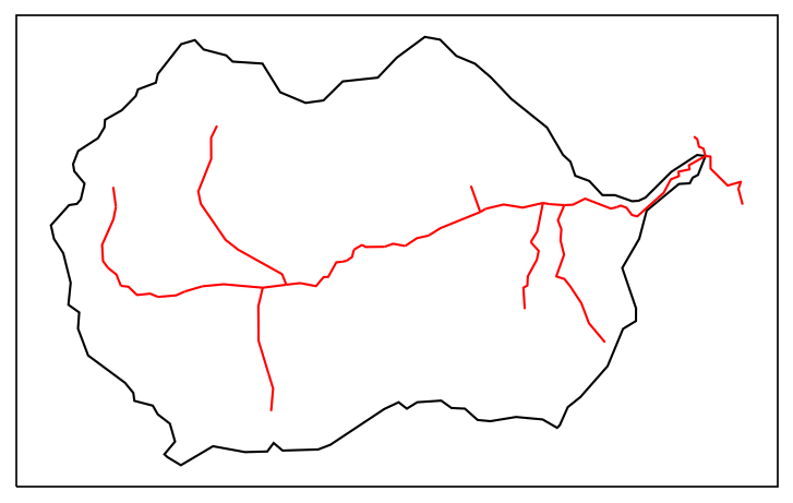
Meshing#
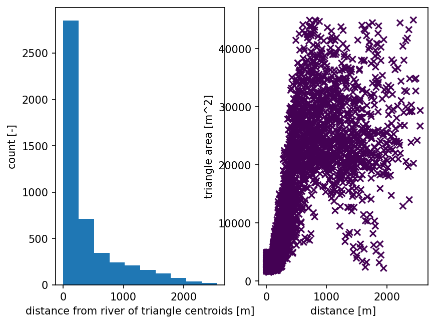
Triangulation refinement: refine triangles if their area (in m^2) is greater than A(d), where d is the distance from the triangle centroid to the nearest stream. A(d) is a piecewise linear function – A = A0 if d <= d0, A = A1 if d >= d1, and linearly interpolates between the two endpoints.
Adjust distance and area parameters to refine triangles.
Be careful with the min triangular area (e.g., <1 m^2) in the meshes. It will likely cause the model to run extremely slowly. You may also receive an error saying the tolerance value (i.e., the minimum node distance) is too small. You can increase the smoothing parameter such as simplify_hucs or simplify_rivers in the above step to make the boundaries smoother and meshes coarser.
# form a triangulation on the shape + river network

# triangulation refinement:
# Refine triangles if their area (in m^2) is greater than A(d), where d is the
# distance from the triangle centroid to the nearest stream.
# A(d) is a piecewise linear function -- A = A0 if d <= d0, A = A1 if d >= d1, and
# linearly interpolates between the two endpoints.
d0 = refine_d0; d1 = refine_d1 # distance in meters
A0 = refine_A0; A1 = refine_A1 # triangular area in m^2
# A0 = 5000; A1 = 50000 # triangular area in m^2
#A0 = 500; A1 = 2500
#A0 = 100; A1 = 500

# Refine triangles if they get too acute
min_angle = 32 # degrees

# make 2D mesh
mesh_points2, mesh_tris, areas, dists = watershed_workflow.triangulate(watershed, rivers,
                                               refine_distance=[d0,A0,d1,A1],
                                               refine_min_angle=min_angle,
                                               diagnostics=True)
2025-07-12 18:35:12,266 - root - INFO:
2025-07-12 18:35:12,270 - root - INFO: Triangulation
2025-07-12 18:35:12,274 - root - INFO: ------------------------------
2025-07-12 18:35:12,320 - root - INFO: Triangulating...
2025-07-12 18:35:12,328 - root - INFO:    97 points and 97 facets
2025-07-12 18:35:12,331 - root - INFO:  checking graph consistency
2025-07-12 18:35:12,333 - root - INFO:  tolerance is set to 1
2025-07-12 18:35:12,350 - root - INFO:  building graph data structures
2025-07-12 18:35:12,362 - root - INFO:  triangle.build...
2025-07-12 18:35:19,857 - root - INFO:   ...built: 2486 mesh points and 4793 triangles
2025-07-12 18:35:19,860 - root - INFO: Plotting triangulation diagnostics
2025-07-12 18:35:22,406 - root - INFO:   min area = 1493.2255859375
2025-07-12 18:35:22,409 - root - INFO:   max area = 44960.84326171875
# get a raster for the elevation map, based on NED
dem_profile, dem = watershed_workflow.get_raster_on_shape(sources['DEM'], watershed.exterior(), crs)

# elevate the triangle nodes to the dem
mesh_points3 = watershed_workflow.elevate(mesh_points2, crs, dem, dem_profile)
2025-07-12 18:35:24,067 - root - INFO:
2025-07-12 18:35:24,070 - root - INFO: Loading Raster
2025-07-12 18:35:24,072 - root - INFO: ------------------------------
2025-07-12 18:35:24,084 - root - INFO: Collecting raster
2025-07-12 18:35:24,156 - root - INFO: Collecting DEMs to tile bounds: [-107.11634327399999, 38.817702882000034, -106.96736783099998, 38.90466788700003]
2025-07-12 18:35:24,163 - root - INFO:   Need:
2025-07-12 18:35:24,166 - root - INFO:     ../../data/dem/USGS_NED_1as_n39_w108.tif
2025-07-12 18:35:24,176 - root - INFO:     ../../data/dem/USGS_NED_1as_n39_w107.tif
2025-07-12 18:35:24,198 - root - INFO: source files already exist!
2025-07-12 18:35:24,445 - root - INFO: ... got raster of shape: (313, 536)
2025-07-12 18:35:24,456 - root - INFO: ... got raster bounds: (-107.11634327399999, 38.90466788700003, -106.96745438510615, 38.81772344247477)
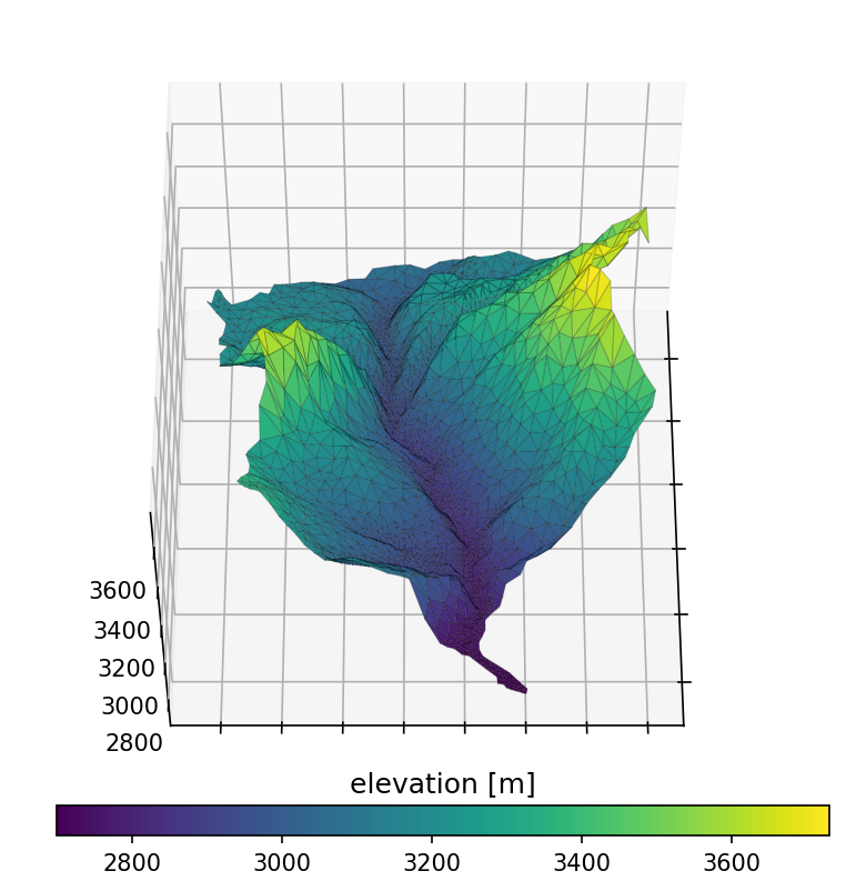
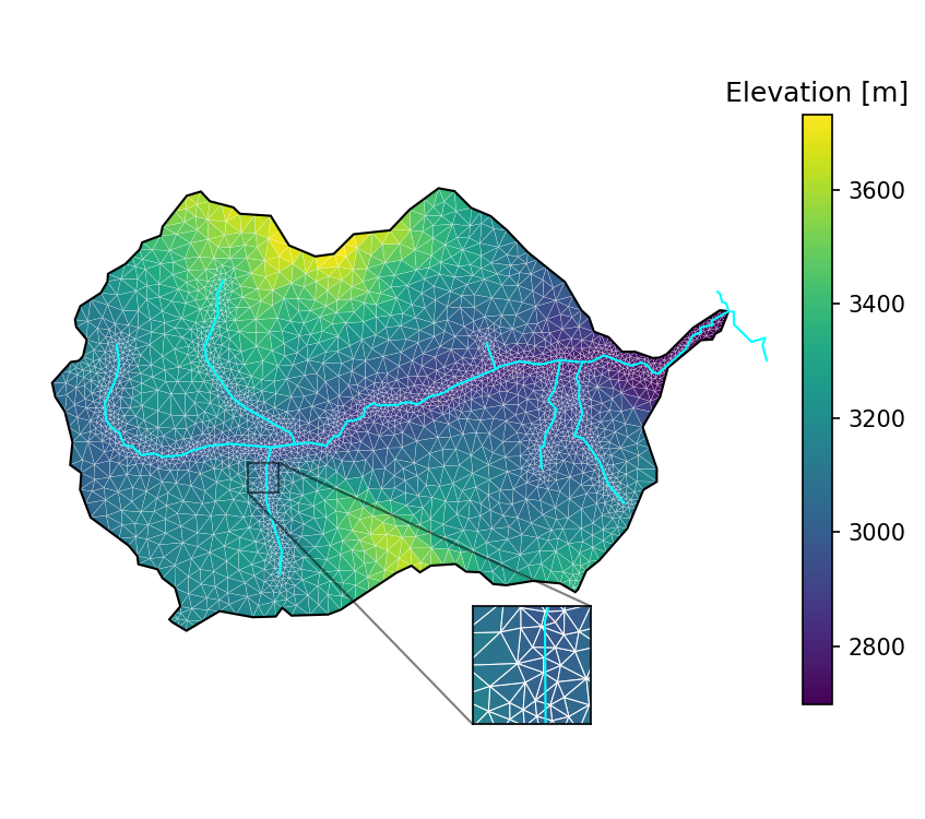
Plotting the resulting mesh can be done in a variety of ways, including both 3D plots and mapview. We show both here, but hereafter use mapview plots as they are a bit clearer (if not so flashy)…
# plot the resulting surface mesh
fig = plt.figure(figsize=figsize_3d)
ax = watershed_workflow.plot.get_ax('3d', fig, window=[0.0,0.2,1,0.8])
cax = fig.add_axes([0.23,0.18,0.58,0.03])

mp = ax.plot_trisurf(mesh_points3[:,0], mesh_points3[:,1], mesh_points3[:,2],
                     triangles=mesh_tris, cmap='viridis',
                     edgecolor=(0,0,0,.2), linewidth=0.5)
cb = fig.colorbar(mp, orientation="horizontal", cax=cax)

t = cax.set_title('elevation [m]')
ax.view_init(55,0)
ax.set_xticklabels(list())
ax.set_yticklabels(list())
[Text(4299000.0, 0, ''),
 Text(4300000.0, 0, ''),
 Text(4301000.0, 0, ''),
 Text(4302000.0, 0, ''),
 Text(4303000.0, 0, ''),
 Text(4304000.0, 0, ''),
 Text(4305000.0, 0, ''),
 Text(4306000.0, 0, ''),
 Text(4307000.0, 0, ''),
 Text(4308000.0, 0, '')]
# plot the resulting surface mesh
fig = plt.figure(figsize=figsize)
ax = watershed_workflow.plot.get_ax(crs, fig, window=[0.05,0.1,0.8,0.8])
#ax2 = workflow.plot.get_ax(crs,fig, window=[0.65,0.05,0.3,0.5])
ax2 = ax.inset_axes([0.58,0.10,0.15,0.15])
cbax = fig.add_axes([.85,0.2,0.03,0.6])

xlim = (320500., 321000.)
ylim = (4302000., 4302500.)

mp = watershed_workflow.plot.triangulation(mesh_points3, mesh_tris, crs, ax=ax,
                                 color='elevation', edgecolor='white', linewidth=0.1)
cbar = fig.colorbar(mp, orientation="vertical", cax=cbax)
watershed_workflow.plot.hucs(watershed, crs, ax=ax, color='k', linewidth=1)
watershed_workflow.plot.rivers(rivers, crs, ax=ax, color='aqua', linewidth=1)
ax.set_aspect('equal', 'datalim')

mp2 = watershed_workflow.plot.triangulation(mesh_points3, mesh_tris, crs, ax=ax2,
                                 color='elevation', edgecolor='white', linewidth=0.5)
watershed_workflow.plot.hucs(watershed, crs, ax=ax2, color='k', linewidth=1)
watershed_workflow.plot.rivers(rivers, crs, ax=ax2, color='aqua', linewidth=1)
ax2.set_xlim(xlim)
ax2.set_ylim(ylim)
ax2.set_xticks([])
ax2.set_yticks([])
ax2.set_aspect('equal', 'datalim')
ax.indicate_inset_zoom(ax2, edgecolor='k')

# add scalebar, use 1 for UTM coordinates, the default unit is "m"
# scalebar1 = ScaleBar(1, location = "lower left", pad=3, frameon=False)
# ax.add_artist(scalebar1)
ax.axis('off')
print(ax.get_xlim())
print(ax.get_ylim())
cbar.ax.set_title('Elevation [m]')
# fig.savefig('../figures/watershed_mesh-2d.jpg',dpi=300)
(316658.3121175361, 329703.25353174284)
(4296859.719285354, 4309904.660699561)
Text(0.5, 1.0, 'Elevation [m]')
# construct the 2D mesh
m2 = watershed_workflow.mesh.Mesh2D(mesh_points3.copy(), list(mesh_tris))
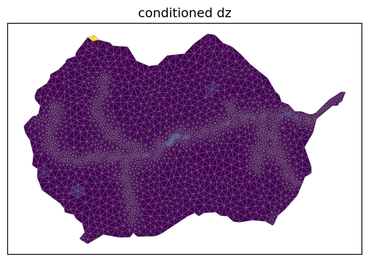
Condition the mesh to remove pits and ponds in the meshes. Advanced tip: use fill_pits_dual(m2, is_waterbody=waterbody_mask) if there exists lakes or reservoirs where pits should not be removed!
# hydrologically condition the mesh, removing pits
watershed_workflow.condition.fill_pits(m2)

# plot the change between the two meshes
diff = np.copy(mesh_points3)
diff[:,2] = m2.points[:,2] - mesh_points3[:,2]
print("max diff = ", np.abs(diff[:,2]).max())
fig, ax = watershed_workflow.plot.get_ax(crs, figsize=figsize)
watershed_workflow.plot.triangulation(diff, m2.conn, crs, color='elevation', edgecolors='gray',
                            linewidth=0.2, ax=ax)
ax.set_title('conditioned dz')
plt.show()
max diff = 93.59001668278142
Add watershed outlet (optional)#
This will add the outlet region in the mesh for better capturing the streamflow in post-processing. Here there is only one catchment with one outlet. However, this may be necessary for watershed with multiple subcatchments with multiple outlets.
list(watershed.polygons())[0].properties
OrderedDict([('OBJECTID', 11223.0),
             ('TNMID', '{C3DA8896-4FF3-4B2F-A382-3B4AFDC6D77E}'),
             ('METASOURCE', None),
             ('SOURCEDATA', None),
             ('SOURCEORIG', None),
             ('SOURCEFEAT', None),
             ('LOADDATE', '2013/01/18 07:08:08.000'),
             ('GNIS_ID', None),
             ('AREAACRES', 13146.76),
             ('AREASQKM', 53.2),
             ('STATES', 'CO'),
             ('HUC12', '140200010204'),
             ('NAME', 'Coal Creek'),
             ('HUTYPE', 'S'),
             ('HUMOD', 'NM'),
             ('TOHUC', '140200010205'),
             ('NONCONTRIB', 0.0),
             ('NONCONTR_1', 0.0),
             ('Shape_Leng', 0.357147902089145),
             ('Shape_Area', 0.005521609626425)])
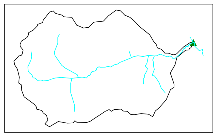
Identify outlets for each catchment. Plot the outlets to verify the correct outlet locations.
Available functions to find the outlets include:
find_outlets_by_crossings(): find all outlets using river network’s crossing points on HUC boundary. This may not work well if river has multiple crossings on the same boundary.find_outlets_by_elevation(): find all outlets by the minimum elevation. This does not work if the minimum elevation within the watershed is not located at the outlet.find_outlets_by_hydroseq(): find outlets using the HydroSequence VAA of NHDPlus. This may take a while.
watershed_workflow.split_hucs.find_outlets_by_elevation(watershed, crs, dem, dem_profile)
# add labeled sets for subcatcprojectnts and outlets.
# Here we use HUC12 code, but any other labels would work.
outlet_width = 500  # half-width (unit is the same as in watershed CRS) to track a labeled set on which to get discharge. Use large values to be conservative.
watershed_polygons = list(watershed.polygons())
catchment_labels = [str(p.properties['HUC12']) for p in watershed_polygons]

watershed_workflow.regions.add_watershed_regions_and_outlets(m2, watershed,
                                                outlet_width=outlet_width,
                                               labels=catchment_labels)
# plot outlets
# fig,ax=plt.subplots(1,1,figsize=(6,4))
fig, ax = watershed_workflow.plot.get_ax(crs, figsize=figsize)
watershed_workflow.plot.hucs(watershed, crs, color='k', outlet_marker = '^', ax =ax, linewidth=1)
watershed_workflow.plot.rivers(rivers, crs,  color='aqua', ax =ax, linewidth=1)
for ls in m2.labeled_sets:
    print(f'{ls.setid} : {ls.entity} : "{ls.name}"')
10000 : CELL : "140200010204"
10001 : CELL : "140200010204 surface"
10002 : FACE : "140200010204 boundary"
10003 : FACE : "140200010204 outlet"
10004 : FACE : "surface domain outlet"
config['catchment_labels'] = catchment_labels
Surface properties#
Meshes interact with data to provide forcing, parameters, and more in the actual simulation. Specifically, we need vegetation type on the surface to provide information about transpiration and subsurface structure to provide information about water retention curves, etc.
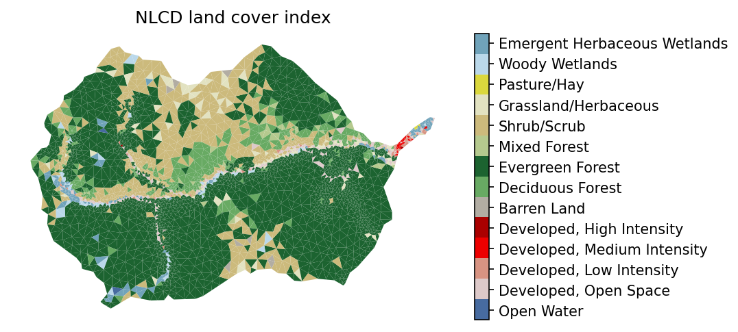
We’ll start by downloading and collecting land cover from the NLCD dataset, and generate sets for each land cover type that cover the surface. Likely these will be some combination of grass, deciduous forest, coniferous forest, and mixed.
Land Cover#
# download the NLCD raster
lc_profile, lc_raster = watershed_workflow.get_raster_on_shape(sources['land cover'],
                                                     watershed.exterior(), crs)

# resample the raster to the triangles
lc = watershed_workflow.values_from_raster(m2.centroids, crs, lc_raster, lc_profile)

# what land cover types did we get?
logging.info('Found land cover dtypes: {}'.format(lc.dtype))
logging.info('Found land cover types: {}'.format(set(lc)))
2025-07-12 18:35:36,701 - root - INFO:
2025-07-12 18:35:36,704 - root - INFO: Loading Raster
2025-07-12 18:35:36,707 - root - INFO: ------------------------------
2025-07-12 18:35:36,711 - root - INFO: Collecting raster
2025-07-12 18:35:37,396 - root - INFO: bounds in my_crs: (-952551.1064432578, 1811083.3381282836, -941371.5911290408, 1818385.78533155)
2025-07-12 18:35:37,408 - root - INFO: ... got raster of shape: (245, 374)
2025-07-12 18:35:37,977 - root - INFO: ... got raster bounds: (-952575.0, 1818405.0, -941355.0, 1811055.0)
2025-07-12 18:35:38,673 - root - INFO: Found land cover dtypes: uint8
2025-07-12 18:35:38,680 - root - INFO: Found land cover types: {71, 41, 42, 43, 11, 81, 52, 21, 22, 23, 24, 90, 31, 95}
# plot the NLCD data

# -- get the NLCD colormap which uses official NLCD colors and labels
nlcd_indices, nlcd_cmap, nlcd_norm, nlcd_ticks, nlcd_labels = \
                watershed_workflow.colors.generate_nlcd_colormap(lc)

# plot the image
fig = plt.figure(figsize=figsize)
ax = watershed_workflow.plot.get_ax(crs, fig)

polys = watershed_workflow.plot.mesh(m2, crs, ax=ax, color=lc, cmap=nlcd_cmap,
                                     norm=nlcd_norm, edgecolor='none',
                                     facecolor='color', linewidth=0.5)
watershed_workflow.colors.colorbar_index(ncolors=len(nlcd_indices), cmap=nlcd_cmap,
                                         labels=nlcd_labels)
ax.set_title("NLCD land cover index")
ax.axis('off')
kwargs =  {'cmap': <matplotlib.colors.ListedColormap object at 0x409569ffd0>, 'norm': <matplotlib.colors.BoundaryNorm object at 0x40956c9060>, 'edgecolor': 'none', 'linewidth': 0.5}
setting face color =  [42 42 95 ... 52 52 52]
(316690.15495, 329034.55405000004, 4299344.3309, 4307420.0490999995)
nlcd_indices, nlcd_labels
([11, 21, 22, 23, 24, 31, 41, 42, 43, 52, 71, 81, 90, 95],
 ['Open Water',
  'Developed, Open Space',
  'Developed, Low Intensity',
  'Developed, Medium Intensity',
  'Developed, High Intensity',
  'Barren Land',
  'Deciduous Forest',
  'Evergreen Forest',
  'Mixed Forest',
  'Shrub/Scrub',
  'Grassland/Herbaceous',
  'Pasture/Hay',
  'Woody Wetlands',
  'Emergent Herbaceous Wetlands'])
# # add labeled sets to the mesh for NLCD
# nlcd_labels_dict = dict(zip(nlcd_indices, nlcd_labels))
# watershed_workflow.mesh.add_nlcd_labeled_sets(m2, lc, nlcd_labels_dict)

# for ls in m2.labeled_sets:
#     print(f'{ls.setid} : {ls.entity} : "{ls.name}"')
LAI#
Download MODIS LAI and LULC, block until it is finished!
NOTE: if you get an error here about MODIS AppEEARs username and password, realize that you must register for a login in the AppEEARs database. See: print(sources['lai'].__doc__)
You may encounter download issues if the files are too big. In that case, manually download the MODIS data using AppEEARS. Here are brief steps:
Sign in if you already registered.
Click
Extract --> AreaClick
Start a new requestUpload the watershed shapefile (in lat-lon). Important: draw a box region surrounding the watershed to avoid downloading no_data!
Choose
Start Date(e.g., 2002-7-1) andEnd Date(e.g., 2021-1-1)Select product for Landcover (e.g.,
MCD12Q1.006) or LAI (e.g.,MCD15A3H.006)Select layers or for landcover (i.e.,
LC_Type1) or LAI (i.e.,Lai_500m). You may choose to include all layers, but not all will be used.Select
NetCDF-4as the output file formatClick
Submit. It will send an email after download is completed.
## Uncomment the next three lines if you want to try downloading through WW
# modis = sources['lai'].get_data(watershed.exterior(), crs, start, end)
# if not isinstance(modis, watershed_workflow.datasets.State):
#     modis = sources['lai'].wait(modis)
modis = sources['lai'].get_data(watershed.exterior(), crs, variables = ['LULC', 'LAI'], filenames=[watershed_modis_lulc, watershed_modis_lai])
2025-07-12 18:35:45,502 - root - INFO: ... reading LULC from ../../data/examples/CoalCreek/sources/land_cover/MODIS/MCD12Q1.006_500m_aid0001.nc
2025-07-12 18:35:45,631 - root - INFO: ... reading LAI from ../../data/examples/CoalCreek/sources/land_cover/MODIS/MCD15A3H.006_500m_aid0001.nc
731
915
# drop data on leap day -- MODIS is real data, but we work with data on a noleap calendar.  This drops Dec 31
for dset in modis.collections:
    watershed_workflow.datasets.removeLeapDay(dset)
<class 'watershed_workflow.datasets.Dataset'> <class 'str'> LULC
<class 'watershed_workflow.datasets.Dataset'> <class 'str'> LAI
# convert Gregorian time to datetime64
modis_times = np.array([np.datetime64(t.strftime('%Y-%m-%d')) for t in modis['LULC'].times])

modis_times
array(['2002-01-01', '2003-01-01', '2004-01-01', '2005-01-01',
       '2006-01-01', '2007-01-01', '2008-01-01', '2009-01-01',
       '2010-01-01', '2011-01-01', '2012-01-01', '2013-01-01',
       '2014-01-01', '2015-01-01', '2016-01-01', '2017-01-01',
       '2018-01-01', '2019-01-01', '2020-01-01'], dtype='datetime64[D]')
# select the year of 2016 for MODIS landcover to match 2016 NLCD land cover
lc_idx = np.where(modis_times == datetime.date(2016, 1, 1))[0][0]
lc_idx
14
# resample the raster to the triangles
modis_lc = watershed_workflow.values_from_raster(m2.centroids, crs, modis['LULC'].data[lc_idx,:,:],
                                                 modis['LULC'].profile)

# what land cover types did we get?
logging.info('Found land cover dtypes: {}'.format(modis_lc.dtype))
logging.info('Found land cover types: {}'.format(set(modis_lc)))
2025-07-12 18:35:46,383 - root - INFO: Found land cover dtypes: int16
2025-07-12 18:35:46,389 - root - INFO: Found land cover types: {8, 9, 10, 1}
assert (np.unique(modis_lc)>0).all(), f"Found negative index: {np.unique(modis_lc)[np.unique(modis_lc)<0]} in landcover types! Double check your MODIS LULC download and make sure it covers a larger area than the watershed (e.g., a box that bounds the watershed)"
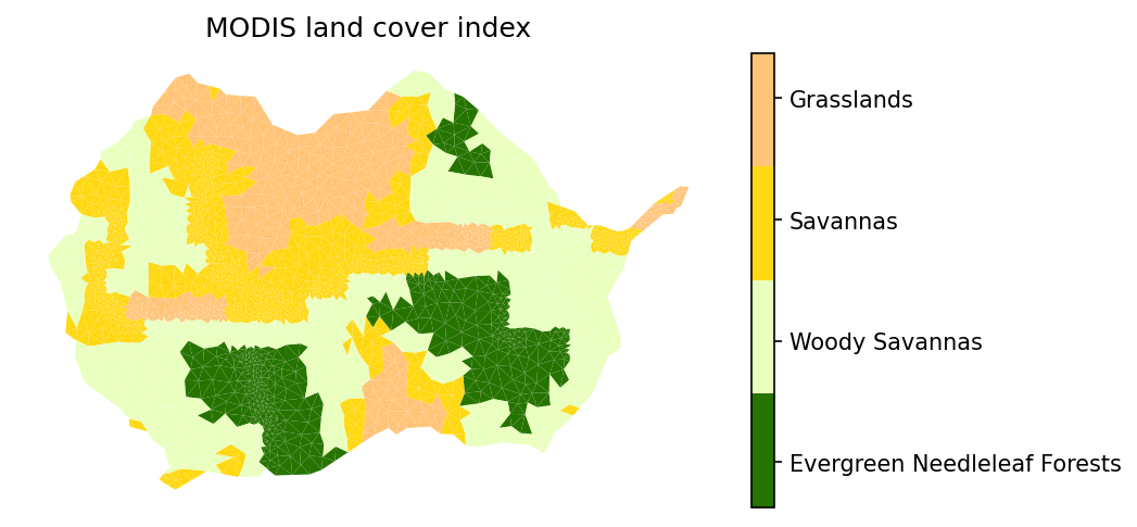
# plot the modis lulc data

# -- get the MODIS colormap which uses official MODIS colors and labels
modis_indices, modis_cmap, modis_norm, modis_ticks, modis_labels = \
                watershed_workflow.colors.generate_modis_colormap(modis_lc)

# plot the image
fig = plt.figure(figsize=figsize)
ax = watershed_workflow.plot.get_ax(crs, fig)

polys = watershed_workflow.plot.mesh(m2, crs, ax=ax, color=modis_lc, cmap=modis_cmap,
                                     norm=modis_norm, edgecolor='none',
                                     facecolor='color', linewidth=0.5)
watershed_workflow.colors.colorbar_index(ncolors=len(modis_indices), cmap=modis_cmap,
                                         labels=modis_labels)
ax.set_title("MODIS land cover index")
ax.axis('off')
kwargs =  {'cmap': <matplotlib.colors.ListedColormap object at 0x4095e6bf40>, 'norm': <matplotlib.colors.BoundaryNorm object at 0x4095e694b0>, 'edgecolor': 'none', 'linewidth': 0.5}
setting face color =  [ 8  8 10 ...  9 10 10]
(316690.15495, 329034.55405000004, 4299344.3309, 4307420.0490999995)
# plot both NLCD and MODIS to form the image cross-correlation
# if generate_plots:
axs = []
fig, a0 = watershed_workflow.plot.get_ax(lc_profile['crs'], nrow=1, ncol=2, index=1, figsize=(15,5))
axs.append(a0)

# plot the image
# -- get the NLCD colormap which uses official NLCD colors and labels
nlcd_indices, nlcd_cmap, nlcd_norm, nlcd_ticks, nlcd_labels = \
            watershed_workflow.colors.generate_nlcd_colormap(np.unique(lc_raster))

im = watershed_workflow.plot.raster(lc_profile, lc_raster, ax=axs[0], cmap=nlcd_cmap, norm=nlcd_norm)
watershed_workflow.plot.shply(watershed_workflow.warp.shply(watershed.exterior(), crs, lc_profile['crs']), lc_profile['crs'], 'k', axs[0])
watershed_workflow.colors.colorbar_index(ncolors=len(np.unique(lc_raster)), cmap=nlcd_cmap, labels=nlcd_labels, ax=axs[0])
axs[0].set_title("NLCD Index")


modis_raster = modis['LULC'].data[-1]
modis_profile = modis['LULC'].profile

a1 = watershed_workflow.plot.get_ax(modis_profile['crs'], nrow=1, ncol=2, index=2, fig=fig)
axs.append(a1)

modis_indices, modis_cmap, modis_norm, modis_ticks, modis_labels = \
            watershed_workflow.colors.generate_modis_colormap(np.unique(modis_raster))
# print(modis_indices, modis_labels)
# print(modis_cmap(8))
# print(modis_cmap(4))
im = watershed_workflow.plot.raster(modis_profile, modis_raster, ax=axs[1], cmap=modis_cmap, norm=modis_norm)
watershed_workflow.plot.shply(watershed_workflow.warp.shply(watershed.exterior(), crs, modis_profile['crs']), modis_profile['crs'], 'k', axs[1])
watershed_workflow.colors.colorbar_index(ncolors=len(np.unique(modis_raster)), cmap=modis_cmap, labels=modis_labels, ax=axs[1])
axs[1].set_title("MODIS LULC Index")
2025-07-12 18:35:53,597 - root - INFO: BOUNDS: (-952575.0, 1811055.0, -941355.0, 1818405.0)
2025-07-12 18:35:55,069 - root - INFO: BOUNDS: (-107.13124999040262, 38.81041666318983, -106.952083323752, 38.91458332984716)
Text(0.5, 1.0, 'MODIS LULC Index')

# determine a crosswalk between NLCD and MODIS -- for each NLCD index,
# what MODIS index correlates best.
crosswalk = watershed_workflow.land_cover_properties.computeMaximalCrosswalkCorrelation(
    modis['LULC'].profile, modis['LULC'].data[lc_idx,:,:], lc_profile, lc_raster)
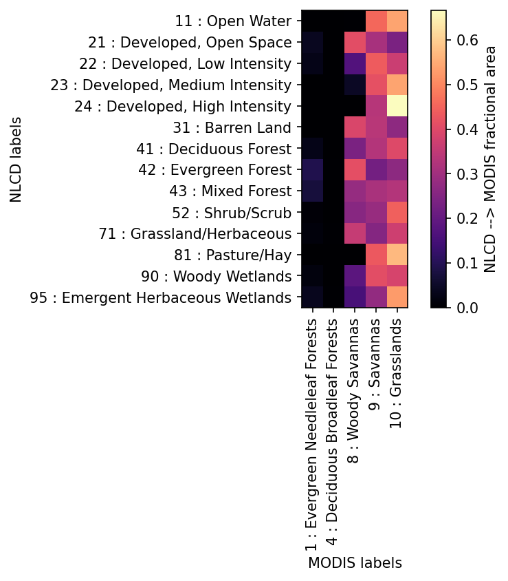
# print the crosswalk.
crosswalk
{11: 10,
 21: 8,
 22: 9,
 23: 10,
 24: 10,
 31: 8,
 41: 10,
 42: 8,
 43: 10,
 52: 10,
 71: 10,
 81: 10,
 90: 9,
 95: 10}
nlcd_color_new = 99 * np.ones_like(lc)

for k,v in crosswalk.items():
    # for label in v:
    # index = sources['land cover'].indices[label]
    nlcd_color_new[np.where(lc == k)] = v
np.unique(nlcd_color_new)
array([ 8, 9, 10], dtype=uint8)
# plot new NLCD data

# -- get the NLCD colormap which uses official NLCD colors and labels
nlcd_indices_new, nlcd_cmap_new, nlcd_norm_new, nlcd_ticks_new, nlcd_labels_new = \
                watershed_workflow.colors.generate_modis_colormap(nlcd_color_new)

# plot the image
fig = plt.figure(figsize=figsize)
ax = watershed_workflow.plot.get_ax(crs, fig)

polys = watershed_workflow.plot.mesh(m2, crs, ax=ax, color=nlcd_color_new, cmap=nlcd_cmap_new,
                                     norm=nlcd_norm_new, edgecolor='none',
                                     facecolor='color', linewidth=0.5)
watershed_workflow.colors.colorbar_index(ncolors=len(nlcd_indices_new), cmap=nlcd_cmap_new,
                                         labels=nlcd_labels_new)
ax.set_title("New land cover index")
ax.axis('off')
/opt/conda/envs/watershed_workflow/lib/python3.10/site-packages/pyproj/crs/crs.py:1282: UserWarning: You will likely lose important projection information when converting to a PROJ string from another format. See: https://proj.org/faq.html#what-is-the-best-format-for-describing-coordinate-reference-systems
  proj = self._crs.to_proj4(version=version)
kwargs =  {'cmap': <matplotlib.colors.ListedColormap object at 0x40961991b0>, 'norm': <matplotlib.colors.BoundaryNorm object at 0x40961998a0>, 'edgecolor': 'none', 'linewidth': 0.5}
setting face color =  [ 8  8 10 ... 10 10 10]
(316690.15495, 329034.55405000004, 4299344.3309, 4307420.0490999995)
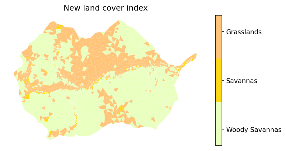
nlcd_indices_new, nlcd_labels_new
([8, 9, 10], ['Woody Savannas', 'Savannas', 'Grasslands'])
# add labeled sets to the mesh for new NLCD
# nlcd_labels_new = ['MODIS ' + i for i in nlcd_labels_new] # comment this to be consistent with the column labels in pandas
nlcd_labels_dict = dict(zip(nlcd_indices_new, nlcd_labels_new))

# Assert that the list does NOT contain 1, 2, or 3
assert all(x not in nlcd_indices_new for x in [1, 2, 3]), "MODIS indices contain 1, 2, or 3, which are reserved labels for surface, bottom and sidesets!"
watershed_workflow.regions.add_nlcd_labeled_sets(m2, nlcd_color_new, nlcd_labels_dict)
config['nlcd_indices'] = [int(i) for i in nlcd_indices_new]
config['nlcd_labels'] = nlcd_labels_new
for ls in m2.labeled_sets:
    print(f'{ls.setid} : {ls.entity} : "{ls.name}"')
10000 : CELL : "140200010204"
10001 : CELL : "140200010204 surface"
10002 : FACE : "140200010204 boundary"
10003 : FACE : "140200010204 outlet"
10004 : FACE : "surface domain outlet"
8 : CELL : "Woody Savannas"
9 : CELL : "Savannas"
10 : CELL : "Grasslands"
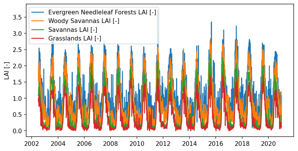
# compute area averaged LAI for each modis land cover
lai_time_series = watershed_workflow.land_cover_properties.computeTimeSeries(
modis['LAI'], modis['LULC'], polygon=watershed.exterior(), polygon_crs=crs)

# # convert Gregorian time to datetime64
# lai_time_series['time [datetime]'] = np.array([np.datetime64(t.strftime('%Y-%m-%d')) for t in lai_time_series['time [datetime]']])

lai_time_series
| time [datetime] | Evergreen Needleleaf Forests LAI [-] | Woody Savannas LAI [-] | Savannas LAI [-] | Grasslands LAI [-] | |
|---|---|---|---|---|---|
| 0 | 2002-07-04 00:00:00 | 1.582051 | 1.531618 | 1.082292 | 0.900000 |
| 1 | 2002-07-08 00:00:00 | 1.864103 | 1.727206 | 1.188542 | 1.007576 |
| 2 | 2002-07-12 00:00:00 | 2.125641 | 1.954412 | 1.343750 | 0.986364 |
| 3 | 2002-07-16 00:00:00 | 2.115385 | 2.102206 | 1.352083 | 1.037879 |
| 4 | 2002-07-20 00:00:00 | 1.505128 | 1.398529 | 0.842708 | 0.748485 |
| ... | ... | ... | ... | ... | ... |
| 1694 | 2020-12-18 00:00:00 | 1.030769 | 1.208824 | 0.483333 | 0.180303 |
| 1695 | 2020-12-22 00:00:00 | 0.589744 | 0.420588 | 0.154167 | 0.178788 |
| 1696 | 2020-12-26 00:00:00 | 0.582051 | 0.550000 | 0.167708 | 0.110606 |
| 1697 | 2020-12-30 00:00:00 | 0.828205 | 0.327941 | 0.188542 | 0.150000 |
| 1698 | 2021-01-01 00:00:00 | 1.082051 | 0.815441 | 0.253125 | 0.136364 |
1699 rows × 5 columns
# # compute area averaged LAI for each modis land cover
# lai_time_series = watershed_workflow.land_cover_properties.computeTimeSeries(
# modis['LAI'], modis['LULC'], unique_lc = unique_modis, lc_idx = lc_idx)
# lai_time_series
# plot LAI
fig,ax = plt.subplots(1,1, figsize=(8,4))
times = np.array([datetime.datetime(t.year, t.month, t.day) for t in lai_time_series['time [datetime]']])

# times = pandas.to_datetime(lai_time_series['time [datetime]'])
for icol in lai_time_series.columns[1:]:
    ax.plot(times, lai_time_series[icol], label = icol)
plt.ylabel("LAI [-]")
ax.legend()
<matplotlib.legend.Legend at 0x40962661a0>
time0_dt = datetime.datetime.strptime(origin_date, "%Y-%m-%d")
time0_cftime = cftime.DatetimeNoLeap(time0_dt.year, time0_dt.month, time0_dt.day)

# write raw LAI to disk
config['LAI_filename'] = os.path.join('..', '..', 'data', 'examples', watershed_name, 'processed', 'watershed_lai_raw.h5')
watershed_workflow.io.write_timeseries_to_hdf5(config['LAI_filename'], lai_time_series,
                                              attributes={'name': 'MODIS LAI based on MODIS LULC',
                                                         'unit': 'none'},
                                               time0=time0_cftime)
2025-07-12 18:36:09,282 - root - INFO: Writing HDF5 file: ../../data/examples/CoalCreek/processed/watershed_lai_raw.h5
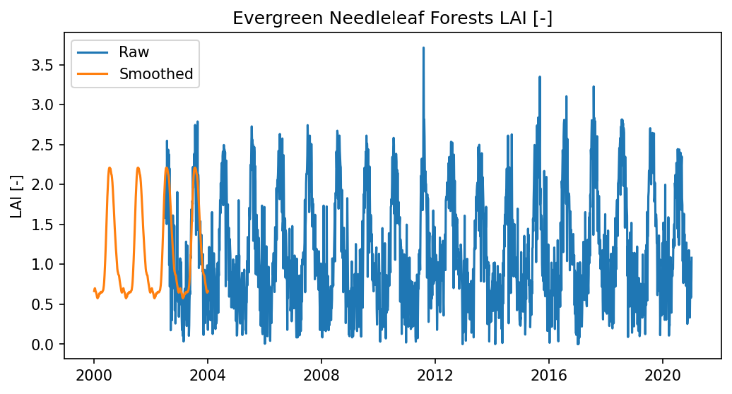
Generate smoothed MODIS LAI data for spinup runs.
# also compute a typical year of LAI
# the start year 2000 can be arbitary since all time are relative in cyclic runs
lai_time_series_smoothed = watershed_workflow.timeseries.computeAverageYear(lai_time_series, output_nyears=nyears_cyclic_steadystate,
                                                                            start_year=2000, smooth=True)
lai_time_series_smoothed
| time [datetime] | Evergreen Needleleaf Forests LAI [-] | Woody Savannas LAI [-] | Savannas LAI [-] | Grasslands LAI [-] | |
|---|---|---|---|---|---|
| 0 | 2000-01-01 00:00:00 | 0.665138 | 0.503850 | 0.185003 | 0.114609 |
| 1 | 2000-01-02 00:00:00 | 0.669486 | 0.504710 | 0.184404 | 0.114643 |
| 2 | 2000-01-03 00:00:00 | 0.675696 | 0.506218 | 0.184019 | 0.114689 |
| 3 | 2000-01-04 00:00:00 | 0.681729 | 0.507545 | 0.183845 | 0.114719 |
| 4 | 2000-01-05 00:00:00 | 0.687301 | 0.508614 | 0.183870 | 0.114705 |
| ... | ... | ... | ... | ... | ... |
| 1455 | 2003-12-27 00:00:00 | 0.662146 | 0.505514 | 0.189364 | 0.115856 |
| 1456 | 2003-12-28 00:00:00 | 0.664010 | 0.505158 | 0.188589 | 0.115406 |
| 1457 | 2003-12-29 00:00:00 | 0.664069 | 0.504498 | 0.187668 | 0.115088 |
| 1458 | 2003-12-30 00:00:00 | 0.662339 | 0.503702 | 0.186626 | 0.114795 |
| 1459 | 2003-12-31 00:00:00 | 0.662727 | 0.503500 | 0.185741 | 0.114648 |
1460 rows × 5 columns
# # compute area averaged LAI for each modis land cover
# # unique_nlcd = list(np.unique(lc))
# unique_modis = modis_indices

# lai_time_series_smoothed = watershed_workflow.land_cover_properties.computeTimeSeries(
# modis['LAI'], modis['LULC'], polygon=watershed_shp, polygon_crs=crs,
#     unique_lc = unique_modis, lc_idx = lc_idx)


# # convert Gregorian time to datetime64
# lai_time_series_smoothed['time [datetime]'] = np.array([np.datetime64(t.strftime('%Y-%m-%d')) for t in lai_time_series_smoothed['time [datetime]']])


# lai_time_series_smoothed
# # compute area averaged LAI for each modis land cover
# lai_time_series_smoothed = watershed_workflow.land_cover_properties.compute_time_series(
# modis['LAI'], modis['LULC'], unique_lc = unique_modis, lc_idx = lc_idx, smooth=True)
# lai_time_series_smoothed
# plot LAI
ilc = lai_time_series.columns[1]
fig,ax = plt.subplots(1,1, figsize=(8,4))
# times = pandas.to_datetime(lai_time_series['time [datetime]'])
new_times = np.array([datetime.datetime(t.year, t.month, t.day) for t in lai_time_series_smoothed['time [datetime]']])

# new_times = pandas.to_datetime(lai_time_series_smoothed['time [datetime]'])

ax.plot(times, lai_time_series[ilc], label = "Raw")
ax.plot(new_times, lai_time_series_smoothed[ilc], label = "Smoothed")
plt.ylabel("LAI [-]")
plt.title(ilc)
ax.legend()
<matplotlib.legend.Legend at 0x4096405180>
# write to disk
config['LAI_typical_filename'] = os.path.join('..', '..', 'data', 'examples', watershed_name, 'processed', 'watershed_lai_typical.h5')
attributes={'name':f'Typical LAI generated MODIS LAI data from {times[0]} to {times[len(times)-1]}, averaged for all days across each year, then repeated for 10 years',
           'origin date':origin_date}

watershed_workflow.io.write_timeseries_to_hdf5(config['LAI_typical_filename'],
                                               lai_time_series_smoothed,
                                               time0=None) # use the first date as the time0, relative time to be consistent with start time in xml file
2025-07-12 18:36:12,317 - root - INFO: Writing HDF5 file: ../../data/examples/CoalCreek/processed/watershed_lai_typical.h5
Subsurface properties#
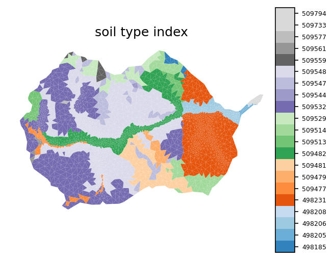
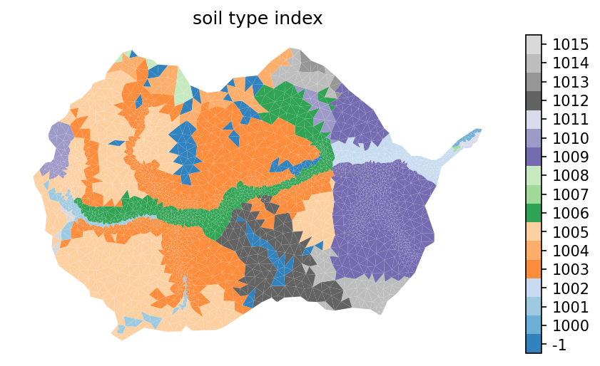
Get soil structure from SSURGO. By soil structure, here we calculate, for each formation identified in SSURGO, a soil depth, porosity, permeability, and percent sand/silt/clay (which are then handed off to Rosetta to get a van Genuchten model).
Below this soil we also identify a geologic layer provided by GLHYMPS. This provides information about the deeper subsurface.
SSURGO Soil Properties#
# download the NRCS soils data as shapes and project it onto the mesh

# -- download the shapes
soil_profile, soil_survey, soil_survey_props = \
        watershed_workflow.get_shapes(sources['soil structure'], [watershed.exterior(),],
                                      crs, crs, properties=True)


# -- determine the NRCS mukey for each soil unit; this uniquely identifies soil
#    properties
soil_ids = np.array(soil_survey_props['mukey'][:], np.int32)

# -- color a raster by the polygons (this makes identifying a triangle's value much
#    more efficient)
soil_color_profile, soil_color_raster = watershed_workflow.color_raster_from_shapes(soil_survey, crs, soil_ids,
                                                                                    watershed.exterior().bounds, 10, crs, -1)

# -- resample the raster to the triangles
soil_color = watershed_workflow.values_from_raster(m2.centroids, crs,
                                         soil_color_raster, soil_color_profile)


soil_color = soil_color.astype(int)
2025-07-12 18:36:12,449 - root - INFO:
2025-07-12 18:36:12,452 - root - INFO: Loading shapes
2025-07-12 18:36:12,455 - root - INFO: ------------------------------
2025-07-12 18:36:12,538 - root - INFO: Attempting to download source for target '../../data/soil_structure/SSURGO/SSURGO_-107.1073_38.8271_-106.9759_38.8957.shp'
2025-07-12 18:36:12,614 - root - INFO:   Found 109 shapes.
2025-07-12 18:36:12,622 - root - INFO:   and crs: epsg:4326
2025-07-12 18:36:12,625 - root - INFO:   Downloaded 109 total shapes
2025-07-12 18:36:12,628 - root - INFO:   Downloaded 32 unique mukeys
2025-07-12 18:36:12,865 - root - INFO: found 32 unique MUKEYs.
2025-07-12 18:36:17,740 - root - INFO: Running Rosetta for van Genutchen parameters
2025-07-12 18:36:18,600 - root - INFO:   ... done
2025-07-12 18:36:18,611 - root - INFO:   requested 28 values
2025-07-12 18:36:18,614 - root - INFO:   got 28 responses
2025-07-12 18:36:18,699 - root - INFO: ... found 32 shapes
2025-07-12 18:36:18,701 - root - INFO: Converting to shapely
2025-07-12 18:36:18,704 - root - INFO:  ... done
2025-07-12 18:36:18,714 - root - INFO: Converting to requested CRS
2025-07-12 18:36:18,916 - root - INFO:  ... done
2025-07-12 18:36:18,925 - root - INFO: Coloring shapes onto raster:
2025-07-12 18:36:18,932 - root - INFO:   of shape: (735, 1124)
2025-07-12 18:36:18,934 - root - INFO:   and 32 independent colors
# plot the soil mukey
indices, cmap, norm, ticks, labels = \
        watershed_workflow.colors.generate_indexed_colormap(soil_color, cmap='tab20c')
fig, ax = watershed_workflow.plot.get_ax(crs, figsize=(5,4), window=[0.,0.,0.7,0.9])
cax = fig.add_axes([0.7,0.05,0.05,0.8])

mp = watershed_workflow.plot.mesh(m2, crs, ax=ax, facecolor='color',
                        linewidth=0, color=soil_color,
                        cmap=cmap, norm=norm
                       )

cbar = watershed_workflow.colors.colorbar_index(ncolors=len(np.unique(soil_color)),
                                                cmap=cmap, labels=labels, cax=cax)
cbar.ax.tick_params(labelsize=6)

ax.set_title('soil type index')
ax.axis('off')
/opt/conda/envs/watershed_workflow/lib/python3.10/site-packages/pyproj/crs/crs.py:1282: UserWarning: You will likely lose important projection information when converting to a PROJ string from another format. See: https://proj.org/faq.html#what-is-the-best-format-for-describing-coordinate-reference-systems
  proj = self._crs.to_proj4(version=version)
kwargs =  {'linewidth': 0, 'cmap': <matplotlib.colors.ListedColormap object at 0x409575f910>, 'norm': <matplotlib.colors.BoundaryNorm object at 0x409575eaa0>}
setting face color =  [509548 509514 509733 ... 509482 509482 509529]
(316690.15495, 329034.55405000004, 4299344.3309, 4307420.0490999995)
# Note this is not just the soil ID, but also soil properties.
# print(soil_survey_props.keys())
soil_survey_props.set_index('mukey', inplace=True)
# only select soils within the watershed
soil_survey_props = soil_survey_props.loc[np.unique(soil_color), :]
soil_survey_props
| residual saturation [-] | Rosetta porosity [-] | van Genuchten alpha [Pa^-1] | van Genuchten n [-] | Rosetta permeability [m^2] | thickness [cm] | permeability [m^2] | porosity [-] | bulk density [g/cm^3] | total sand pct [%] | total silt pct [%] | total clay pct [%] | source | |
|---|---|---|---|---|---|---|---|---|---|---|---|---|---|
| mukey | |||||||||||||
| 498185 | 0.240269 | 0.502882 | 0.000092 | 1.319916 | 3.617805e-13 | 152.000000 | 2.279759e-13 | 0.265563 | 1.207632 | 32.946001 | 24.529703 | 42.524296 | NRCS |
| 498205 | 0.181598 | 0.399993 | 0.000139 | 1.457559 | 4.938634e-13 | 152.000000 | 2.734080e-12 | 0.159737 | 1.413553 | 63.518421 | 22.988158 | 13.493421 | NRCS |
| 498206 | 0.181598 | 0.399993 | 0.000139 | 1.457559 | 4.938634e-13 | 152.000000 | 2.734080e-12 | 0.159737 | 1.413553 | 63.518421 | 22.988158 | 13.493421 | NRCS |
| 498208 | 0.208316 | 0.428990 | 0.000071 | 1.420938 | 2.830658e-13 | 152.000000 | 1.184189e-12 | 0.185986 | 1.302697 | 40.662797 | 38.201188 | 21.136015 | NRCS |
| 498231 | 0.213285 | 0.466663 | 0.000059 | 1.416784 | 3.782943e-13 | 107.000000 | 7.331979e-13 | 0.403218 | 1.197010 | 32.639846 | 41.078960 | 26.281194 | NRCS |
| 509477 | 0.175133 | 0.567740 | 0.000103 | 1.383180 | 2.438575e-12 | 152.000000 | 3.039095e-12 | 0.428779 | 0.807465 | 62.072368 | 17.973684 | 19.953947 | NRCS |
| 509479 | 0.230885 | 0.378365 | 0.000079 | 1.374540 | 1.031721e-13 | 125.000000 | 3.172415e-12 | NaN | 1.524444 | 39.279352 | 38.916498 | 21.804150 | NRCS |
| 509481 | 0.230885 | 0.378365 | 0.000079 | 1.374540 | 1.031721e-13 | 125.000000 | 3.172415e-12 | NaN | 1.524444 | 39.279352 | 38.916498 | 21.804150 | NRCS |
| 509482 | 0.207877 | 0.369886 | 0.000092 | 1.397760 | 1.474479e-13 | 120.500000 | 4.654687e-12 | NaN | 1.530585 | 45.389069 | 37.890283 | 16.720648 | NRCS |
| 509513 | 0.219597 | 0.445168 | 0.000072 | 1.395746 | 2.727324e-13 | 152.000000 | 9.122162e-13 | 0.237423 | 1.280039 | 38.422252 | 35.742028 | 25.835720 | NRCS |
| 509514 | 0.241801 | 0.474101 | 0.000079 | 1.340429 | 2.435161e-13 | 152.000000 | 2.375523e-13 | 0.271630 | 1.274496 | 30.592982 | 31.535307 | 37.871711 | NRCS |
| 509529 | 0.196811 | 0.356163 | 0.000157 | 1.406091 | 2.260935e-13 | 152.000000 | 5.850942e-12 | NaN | 1.607097 | 63.571711 | 22.369079 | 14.059211 | NRCS |
| 509532 | 0.199783 | 0.412306 | 0.000087 | 1.422578 | 2.966015e-13 | 152.000000 | 1.526682e-12 | 0.182238 | 1.356006 | 47.934946 | 34.134907 | 17.930147 | NRCS |
| 509544 | NaN | NaN | NaN | NaN | NaN | 152.000000 | 7.000000e-15 | NaN | NaN | NaN | NaN | NaN | NRCS |
| 509547 | NaN | NaN | NaN | NaN | NaN | 152.000000 | 4.230700e-11 | NaN | 2.030000 | NaN | NaN | NaN | NRCS |
| 509548 | 0.189314 | 0.404765 | 0.000104 | 1.433685 | 3.617371e-13 | 152.000000 | 2.006536e-12 | 0.193350 | 1.379123 | 53.676535 | 31.072368 | 15.251096 | NRCS |
| 509559 | 0.210870 | 0.420608 | 0.000078 | 1.410010 | 2.516507e-13 | 61.812500 | 7.504374e-13 | 0.151250 | 1.341513 | 43.240132 | 35.652961 | 21.106908 | NRCS |
| 509561 | 0.246665 | 0.467696 | 0.000081 | 1.332817 | 2.088819e-13 | 139.647059 | 1.590777e-13 | 0.218625 | 1.305591 | 30.228443 | 31.026630 | 38.744927 | NRCS |
| 509577 | NaN | NaN | NaN | NaN | NaN | 152.000000 | NaN | NaN | NaN | NaN | NaN | NaN | NRCS |
| 509733 | 0.157366 | 0.400499 | 0.000221 | 1.762072 | 1.819618e-12 | 86.000000 | 5.262229e-12 | 0.449752 | 1.423158 | 82.200000 | 9.300000 | 8.500000 | NRCS |
| 509794 | 0.220962 | 0.383130 | 0.000140 | 1.367408 | 2.004353e-13 | 152.000000 | 1.554090e-12 | 0.415245 | 1.545395 | 60.571711 | 18.441447 | 20.986842 | NRCS |
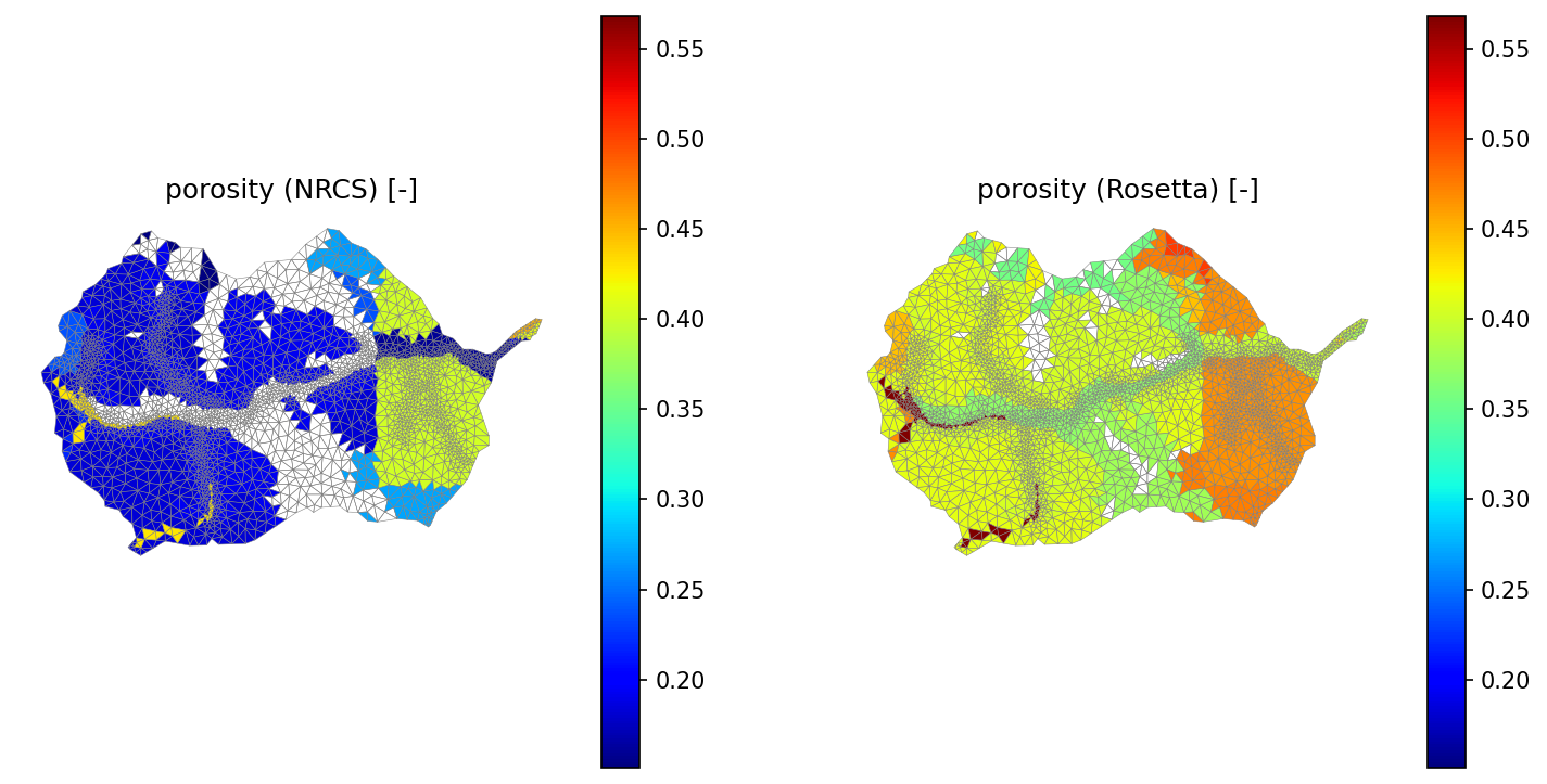
# To demonstrate what we mean by this, plot the porosity of the soil column.
porosity_nrcs = np.empty(soil_color.shape, 'd')
porosity_rosetta = np.empty(soil_color.shape, 'd')

for mukey in soil_survey_props.index:
    porosity_nrcs[soil_color == mukey] = soil_survey_props.loc[mukey, 'porosity [-]']
    porosity_rosetta[soil_color == mukey] = soil_survey_props.loc[mukey, 'Rosetta porosity [-]']

pmin = min(np.nanmin(porosity_nrcs), np.nanmin(porosity_rosetta))
pmax = max(np.nanmax(porosity_nrcs), np.nanmax(porosity_rosetta))
print('min, max = ', pmin, pmax)

fig = plt.figure(figsize=(12,6))
ax1 = watershed_workflow.plot.get_ax(crs, fig, nrow=1, ncol=2, index=1)
mp = watershed_workflow.plot.triangulation(mesh_points3, mesh_tris, crs, ax=ax1,
                color=porosity_nrcs, edgecolor='gray', cmap='jet',
                                           vmin=pmin, vmax=pmax)
cbar = fig.colorbar(mp)
ax1.set_title('porosity (NRCS) [-]')
ax1.axis('off')


ax2 = watershed_workflow.plot.get_ax(crs, fig, nrow=1, ncol=2, index=2)
mp = watershed_workflow.plot.triangulation(mesh_points3, mesh_tris, crs, ax=ax2,
                                 color=porosity_rosetta, edgecolor='gray', cmap='jet', vmin=pmin, vmax=pmax)
cbar = fig.colorbar(mp)
ax2.set_title('porosity (Rosetta) [-]')
ax2.axis('off')
min, max = 0.15125 0.567739729619314
/opt/conda/envs/watershed_workflow/lib/python3.10/site-packages/pyproj/crs/crs.py:1282: UserWarning: You will likely lose important projection information when converting to a PROJ string from another format. See: https://proj.org/faq.html#what-is-the-best-format-for-describing-coordinate-reference-systems
  proj = self._crs.to_proj4(version=version)
(316690.15495, 329034.55405000004, 4299344.3309, 4307420.0490999995)
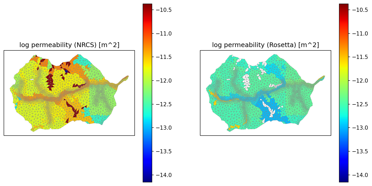
# averaging permeability is a tricky beast.  we average in log space, check that
# unit conversions make sense
fig = plt.figure(figsize=(12,6))
soil_perm_nrcs = np.empty(soil_color.shape, 'd')
soil_perm_rosetta = np.empty(soil_color.shape, 'd')

for mukey in soil_survey_props.index:
    soil_perm_nrcs[soil_color == mukey] = soil_survey_props.loc[mukey, 'permeability [m^2]']
    soil_perm_rosetta[soil_color == mukey] = soil_survey_props.loc[mukey, 'Rosetta permeability [m^2]']

pmin = min(np.nanmin(np.log10(soil_perm_nrcs)), np.nanmin(np.log10(soil_perm_rosetta).min()))
pmax = max(np.nanmax(np.log10(soil_perm_nrcs)), np.nanmax(np.log10(soil_perm_rosetta).max()))


print(f'min = {pmin}, max = {pmax}')

ax1 = watershed_workflow.plot.get_ax(crs, fig, nrow=1, ncol=2, index=1)
mp = watershed_workflow.plot.triangulation(mesh_points3, mesh_tris, crs, ax=ax1,
                                 color=np.log10(soil_perm_nrcs), edgecolor='gray', cmap='jet',
                                vmin=pmin, vmax=pmax)
cbar = fig.colorbar(mp)
ax1.set_title('log permeability (NRCS) [m^2]')

ax2 = watershed_workflow.plot.get_ax(crs, fig, nrow=1, ncol=2, index=2)
mp = watershed_workflow.plot.triangulation(mesh_points3, mesh_tris, crs, ax=ax2,
                                 color=np.log10(soil_perm_rosetta), edgecolor='gray', cmap='jet',
                                vmin=pmin, vmax=pmax)
cbar = fig.colorbar(mp)
ax2.set_title('log permeability (Rosetta) [m^2]')
/tmp/ipykernel_555/45597466.py:11: RuntimeWarning: All-NaN axis encountered
  pmin = min(np.nanmin(np.log10(soil_perm_nrcs)), np.nanmin(np.log10(soil_perm_rosetta).min()))
/tmp/ipykernel_555/45597466.py:12: RuntimeWarning: All-NaN axis encountered
  pmax = max(np.nanmax(np.log10(soil_perm_nrcs)), np.nanmax(np.log10(soil_perm_rosetta).max()))
min = -14.154901959985743, max = -10.373587769507715
Text(0.5, 1.0, 'log permeability (Rosetta) [m^2]')
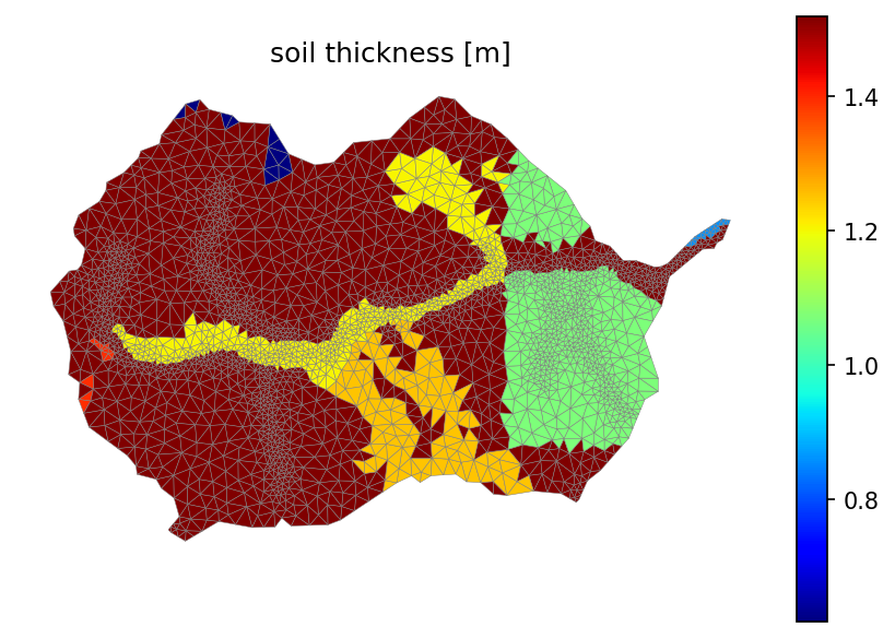
# finally, let's look at the soil thickness, which will define the depth of this layer
soil_thickness = np.zeros(soil_color.shape, 'd')
for mukey in soil_survey_props.index:
    soil_thickness[soil_color == mukey] = soil_survey_props.loc[mukey, 'thickness [cm]']

# print(soil_thickness)
soil_thickness = soil_thickness / 100 # convert cm to m
fig, ax = watershed_workflow.plot.get_ax(crs)
mp = watershed_workflow.plot.triangulation(mesh_points3, mesh_tris, crs, ax=ax,
                                 color=soil_thickness, edgecolor='gray', cmap='jet')
ax.set_title('soil thickness [m]')
cb = fig.colorbar(mp, fraction=0.04, pad=0.04)
ax.axis('off')

print(f'Median soil thickness = {np.nanmedian(soil_thickness)} [m]')
Median soil thickness = 1.52 [m]
def reindex_remove_duplicates(df, index=None):
    """Removes duplicates, creating a new index and saving the old index as tuples of duplicate values. In place!"""
    if index is not None:
        if index in df:
            df.set_index(index, drop=True, inplace=True)

    index_name = df.index.name

    # identify duplicate rows, use all cols as duplicate target
    duplicates = list(df.groupby(list(df)).apply(lambda x: tuple(x.index)))

    # order is preserved
    df.drop_duplicates(inplace=True)
    df.reset_index(inplace=True)
    df[index_name] = duplicates
    return
def replace_column_nans(df, col_nan, col_replacement):
    """In a df, replace col_nan entries by col_replacement if is nan.  In Place!"""
    row_indexer = df[col_nan].isna()
    df.loc[row_indexer, col_nan] = df.loc[row_indexer, col_replacement]
    return
# Note the missing data (white).  This is because some SSURGO map units have no formation with complete
# information.  So we merge the above available data, filling where possible and dropping regions that
# do not have a complete set of properties.
# soil_survey_props_clean = soil_survey_props.copy()
soil_survey_props_clean = soil_survey_props.reset_index()

# later scripts expect 'native_index' as a standard name of holding onto the original IDs
# soil_survey_props_clean.rename_axis('native_index', inplace=True)
soil_survey_props_clean.rename(columns={'mukey':'native_index'}, inplace=True)

# need thickness in m
soil_survey_props_clean['thickness [cm]'] = soil_survey_props_clean['thickness [cm]']/100.
soil_survey_props_clean.rename(columns={'thickness [cm]':'thickness [m]'}, inplace=True)

# where poro or perm is nan, put Rosetta poro
replace_column_nans(soil_survey_props_clean, 'porosity [-]', 'Rosetta porosity [-]')
replace_column_nans(soil_survey_props_clean, 'permeability [m^2]', 'Rosetta permeability [m^2]')

# drop unnecessary columns
for col in ['Rosetta porosity [-]', 'Rosetta permeability [m^2]', 'bulk density [g/cm^3]', 'total sand pct [%]',
            'total silt pct [%]', 'total clay pct [%]']:
    soil_survey_props_clean.pop(col)

soil_survey_props_clean
| native_index | residual saturation [-] | van Genuchten alpha [Pa^-1] | van Genuchten n [-] | thickness [m] | permeability [m^2] | porosity [-] | source | |
|---|---|---|---|---|---|---|---|---|
| 0 | 498185 | 0.240269 | 0.000092 | 1.319916 | 1.520000 | 2.279759e-13 | 0.265563 | NRCS |
| 1 | 498205 | 0.181598 | 0.000139 | 1.457559 | 1.520000 | 2.734080e-12 | 0.159737 | NRCS |
| 2 | 498206 | 0.181598 | 0.000139 | 1.457559 | 1.520000 | 2.734080e-12 | 0.159737 | NRCS |
| 3 | 498208 | 0.208316 | 0.000071 | 1.420938 | 1.520000 | 1.184189e-12 | 0.185986 | NRCS |
| 4 | 498231 | 0.213285 | 0.000059 | 1.416784 | 1.070000 | 7.331979e-13 | 0.403218 | NRCS |
| 5 | 509477 | 0.175133 | 0.000103 | 1.383180 | 1.520000 | 3.039095e-12 | 0.428779 | NRCS |
| 6 | 509479 | 0.230885 | 0.000079 | 1.374540 | 1.250000 | 3.172415e-12 | 0.378365 | NRCS |
| 7 | 509481 | 0.230885 | 0.000079 | 1.374540 | 1.250000 | 3.172415e-12 | 0.378365 | NRCS |
| 8 | 509482 | 0.207877 | 0.000092 | 1.397760 | 1.205000 | 4.654687e-12 | 0.369886 | NRCS |
| 9 | 509513 | 0.219597 | 0.000072 | 1.395746 | 1.520000 | 9.122162e-13 | 0.237423 | NRCS |
| 10 | 509514 | 0.241801 | 0.000079 | 1.340429 | 1.520000 | 2.375523e-13 | 0.271630 | NRCS |
| 11 | 509529 | 0.196811 | 0.000157 | 1.406091 | 1.520000 | 5.850942e-12 | 0.356163 | NRCS |
| 12 | 509532 | 0.199783 | 0.000087 | 1.422578 | 1.520000 | 1.526682e-12 | 0.182238 | NRCS |
| 13 | 509544 | NaN | NaN | NaN | 1.520000 | 7.000000e-15 | NaN | NRCS |
| 14 | 509547 | NaN | NaN | NaN | 1.520000 | 4.230700e-11 | NaN | NRCS |
| 15 | 509548 | 0.189314 | 0.000104 | 1.433685 | 1.520000 | 2.006536e-12 | 0.193350 | NRCS |
| 16 | 509559 | 0.210870 | 0.000078 | 1.410010 | 0.618125 | 7.504374e-13 | 0.151250 | NRCS |
| 17 | 509561 | 0.246665 | 0.000081 | 1.332817 | 1.396471 | 1.590777e-13 | 0.218625 | NRCS |
| 18 | 509577 | NaN | NaN | NaN | 1.520000 | NaN | NaN | NRCS |
| 19 | 509733 | 0.157366 | 0.000221 | 1.762072 | 0.860000 | 5.262229e-12 | 0.449752 | NRCS |
| 20 | 509794 | 0.220962 | 0.000140 | 1.367408 | 1.520000 | 1.554090e-12 | 0.415245 | NRCS |
# drop nans
# soil id with missing properties will be removed, and the space will be filled by geology from below (see mesh extrusion)!
soil_survey_props_clean.dropna(inplace=True)
soil_survey_props_clean.reset_index(drop=True, inplace=True)

# remove duplicates
reindex_remove_duplicates(soil_survey_props_clean, 'native_index')

# assert soil_survey_props_clean['porosity [-]'][:].min() >= min_porosity
# assert soil_survey_props_clean['permeability [m^2]'][:].max() <= max_permeability
soil_survey_props_clean
/tmp/ipykernel_555/2530005601.py:10: DeprecationWarning: DataFrameGroupBy.apply operated on the grouping columns. This behavior is deprecated, and in a future version of pandas the grouping columns will be excluded from the operation. Either pass `include_groups=False` to exclude the groupings or explicitly select the grouping columns after groupby to silence this warning.
  duplicates = list(df.groupby(list(df)).apply(lambda x: tuple(x.index)))
| native_index | residual saturation [-] | van Genuchten alpha [Pa^-1] | van Genuchten n [-] | thickness [m] | permeability [m^2] | porosity [-] | source | |
|---|---|---|---|---|---|---|---|---|
| 0 | (509733,) | 0.240269 | 0.000092 | 1.319916 | 1.520000 | 2.279759e-13 | 0.265563 | NRCS |
| 1 | (509477,) | 0.181598 | 0.000139 | 1.457559 | 1.520000 | 2.734080e-12 | 0.159737 | NRCS |
| 2 | (498205, 498206) | 0.208316 | 0.000071 | 1.420938 | 1.520000 | 1.184189e-12 | 0.185986 | NRCS |
| 3 | (509548,) | 0.213285 | 0.000059 | 1.416784 | 1.070000 | 7.331979e-13 | 0.403218 | NRCS |
| 4 | (509529,) | 0.175133 | 0.000103 | 1.383180 | 1.520000 | 3.039095e-12 | 0.428779 | NRCS |
| 5 | (509532,) | 0.230885 | 0.000079 | 1.374540 | 1.250000 | 3.172415e-12 | 0.378365 | NRCS |
| 6 | (509482,) | 0.207877 | 0.000092 | 1.397760 | 1.205000 | 4.654687e-12 | 0.369886 | NRCS |
| 7 | (498208,) | 0.219597 | 0.000072 | 1.395746 | 1.520000 | 9.122162e-13 | 0.237423 | NRCS |
| 8 | (509559,) | 0.241801 | 0.000079 | 1.340429 | 1.520000 | 2.375523e-13 | 0.271630 | NRCS |
| 9 | (498231,) | 0.196811 | 0.000157 | 1.406091 | 1.520000 | 5.850942e-12 | 0.356163 | NRCS |
| 10 | (509513,) | 0.199783 | 0.000087 | 1.422578 | 1.520000 | 1.526682e-12 | 0.182238 | NRCS |
| 11 | (509794,) | 0.189314 | 0.000104 | 1.433685 | 1.520000 | 2.006536e-12 | 0.193350 | NRCS |
| 12 | (509479, 509481) | 0.210870 | 0.000078 | 1.410010 | 0.618125 | 7.504374e-13 | 0.151250 | NRCS |
| 13 | (498185,) | 0.246665 | 0.000081 | 1.332817 | 1.396471 | 1.590777e-13 | 0.218625 | NRCS |
| 14 | (509514,) | 0.157366 | 0.000221 | 1.762072 | 0.860000 | 5.262229e-12 | 0.449752 | NRCS |
| 15 | (509561,) | 0.220962 | 0.000140 | 1.367408 | 1.520000 | 1.554090e-12 | 0.415245 | NRCS |
# create a new soil_color, keeping on those that are kept here and re-indexing to ATS indices
soil_color_new = -np.ones_like(soil_color)
for new_id, mukeys in enumerate(soil_survey_props_clean['native_index']):
    for mukey in mukeys:
        soil_color_new[np.where(soil_color == mukey)] = 1000+new_id

# # make sure no -1 in soil ids
# assert -1 not in np.unique(soil_color_new)

# image the new soil_color
indices, cmap, norm, ticks, labels = watershed_workflow.colors.generate_indexed_colormap(soil_color_new, cmap='tab20c')
fig, ax = watershed_workflow.plot.get_ax(crs)

mp = watershed_workflow.plot.mesh(m2, crs, ax=ax, facecolor='color',
                        linewidth=0, color=soil_color_new,
                        cmap=cmap, norm=norm)

watershed_workflow.colors.colorbar_index(ncolors=len(np.unique(soil_color_new)), cmap=cmap, labels=labels)

ax.set_title('soil type index')
ax.axis('off')
/opt/conda/envs/watershed_workflow/lib/python3.10/site-packages/pyproj/crs/crs.py:1282: UserWarning: You will likely lose important projection information when converting to a PROJ string from another format. See: https://proj.org/faq.html#what-is-the-best-format-for-describing-coordinate-reference-systems
  proj = self._crs.to_proj4(version=version)
kwargs =  {'linewidth': 0, 'cmap': <matplotlib.colors.ListedColormap object at 0x409c0bc400>, 'norm': <matplotlib.colors.BoundaryNorm object at 0x409c0bc340>}
setting face color =  [1003 1014 1000 ... 1006 1006 1004]
(316690.15495, 329034.55405000004, 4299344.3309, 4307420.0490999995)
GLHYMPS geologic layer#
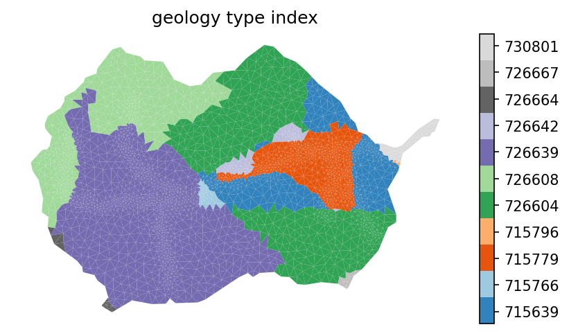
A copy of GLHYMPS v2 geologic shapefile has to be manually downloaded before running the following scripts (see source section for download instructions).
This will get properties (i.e., permeability and porosity) for each geologic layer. In case of missing data, default values of permeability (inf?) and porosity (0.01) will be used. Default van Genuchten alpha, n, and residual saturation are used due to lack of soil/silt/clay pct information.
# extract the GLYHMPS geologic structure data as shapes and project it onto the mesh
target_bounds = watershed.exterior().bounds
logging.info('target bounds: {}'.format(target_bounds))

_, geo_survey, geo_survey_props = \
    watershed_workflow.get_shapes(sources['geologic structure'], target_bounds,
                                  crs, crs, properties=True)

# -- log the bounds targetted and found
logging.info('shape union bounds: {}'.format(
    shapely.ops.cascaded_union(geo_survey).bounds))

# -- determine the ID for each soil unit; this uniquely identifies formation
#    properties
geo_ids = np.array([shp.properties['id'] for shp in geo_survey], np.int32)

# -- color a raster by the polygons (this makes identifying a triangle's value much
#    more efficient)
geo_color_profile, geo_color_raster = \
            watershed_workflow.color_raster_from_shapes(geo_survey, crs, geo_ids,
                                                        target_bounds, 10, crs, -1)

# -- resample the raster to the triangles
geo_color = watershed_workflow.values_from_raster(m2.centroids, crs,
                                         geo_color_raster, geo_color_profile)
2025-07-12 18:36:43,335 - root - INFO: target bounds: (317251.2640131897, 4299711.408984916, 328473.4449929282, 4307052.970983125)
2025-07-12 18:36:43,339 - root - INFO:
2025-07-12 18:36:43,342 - root - INFO: Loading shapes
2025-07-12 18:36:43,344 - root - INFO: ------------------------------
2025-07-12 18:36:43,346 - root - INFO: Getting shapes of GLHYMPS on bounds: (317251.2640131897, 4299711.408984916, 328473.4449929282, 4307052.970983125)
2025-07-12 18:36:43,624 - root - INFO: ... found 17 shapes
2025-07-12 18:36:43,626 - root - INFO: Converting to shapely
2025-07-12 18:36:43,678 - root - INFO:  ... done
2025-07-12 18:36:43,684 - root - INFO: Converting to requested CRS
2025-07-12 18:36:43,841 - root - INFO:  ... done
2025-07-12 18:36:43,910 - root - INFO: shape union bounds: (309452.03384970897, 4277422.824854818, 338890.05886956863, 4329709.205645651)
2025-07-12 18:36:43,914 - root - INFO: Coloring shapes onto raster:
2025-07-12 18:36:43,921 - root - INFO:   of shape: (735, 1124)
2025-07-12 18:36:43,924 - root - INFO:   and 17 independent colors
geo_color = geo_color.astype(int)
geo_survey_props.set_index('id', inplace=True)
geo_survey_props = geo_survey_props.loc[np.unique(geo_color), :]
geo_survey_props
| source | permeability [m^2] | logk_stdev [-] | porosity [-] | van Genuchten alpha [Pa^-1] | van Genuchten n [-] | residual saturation [-] | |
|---|---|---|---|---|---|---|---|
| id | |||||||
| 715639 | GLHYMPS | 6.309573e-16 | 2.50 | 0.19 | 0.000025 | 2.0 | 0.01 |
| 715766 | GLHYMPS | 3.162278e-13 | 1.80 | 0.09 | 0.000817 | 2.0 | 0.01 |
| 715779 | GLHYMPS | 1.000000e-13 | 2.00 | 0.22 | 0.000294 | 2.0 | 0.01 |
| 715796 | GLHYMPS | 6.309573e-16 | 2.50 | 0.19 | 0.000025 | 2.0 | 0.01 |
| 726604 | GLHYMPS | 6.309573e-16 | 2.50 | 0.19 | 0.000025 | 2.0 | 0.01 |
| 726608 | GLHYMPS | 6.309573e-16 | 2.50 | 0.19 | 0.000025 | 2.0 | 0.01 |
| 726639 | GLHYMPS | 3.162278e-13 | 1.80 | 0.09 | 0.000817 | 2.0 | 0.01 |
| 726642 | GLHYMPS | 1.000000e-13 | 2.00 | 0.22 | 0.000294 | 2.0 | 0.01 |
| 726664 | GLHYMPS | 1.000000e-13 | 2.00 | 0.22 | 0.000294 | 2.0 | 0.01 |
| 726667 | GLHYMPS | 3.162278e-13 | 1.80 | 0.09 | 0.000817 | 2.0 | 0.01 |
| 730801 | GLHYMPS | 3.019952e-11 | 1.61 | 0.01 | 0.023953 | 2.0 | 0.01 |
# plot the geologic formation id
fig = plt.figure(figsize=figsize)
ax = watershed_workflow.plot.get_ax(crs, fig)

indices, cmap, norm, ticks, labels = watershed_workflow.colors.generate_indexed_colormap(geo_color, cmap = 'tab20c')


mp = watershed_workflow.plot.mesh(m2, crs, ax=ax, facecolor='color',
                                 linewidth=0, color=geo_color, cmap=cmap, norm=norm)

watershed_workflow.colors.colorbar_index(ncolors=len(np.unique(geo_color)), cmap=cmap, labels = labels)

ax.set_title('geology type index')
ax.axis('off')
/opt/conda/envs/watershed_workflow/lib/python3.10/site-packages/pyproj/crs/crs.py:1282: UserWarning: You will likely lose important projection information when converting to a PROJ string from another format. See: https://proj.org/faq.html#what-is-the-best-format-for-describing-coordinate-reference-systems
  proj = self._crs.to_proj4(version=version)
kwargs =  {'linewidth': 0, 'cmap': <matplotlib.colors.ListedColormap object at 0x409607de70>, 'norm': <matplotlib.colors.BoundaryNorm object at 0x409607da20>}
setting face color =  [726639 726667 730801 ... 726604 726604 726608]
(316690.15495, 329034.55405000004, 4299344.3309, 4307420.0490999995)
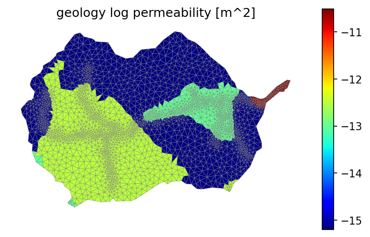
# averaging permeability is a tricky beast.  we average in log space, check that unit conversions make sense
fig = plt.figure(figsize=(12,6))
geol_perm = np.empty(geo_color.shape, 'd')
# soil_perm_rosetta = np.empty(soil_color.shape, 'd')

for i in geo_survey_props.index:
    geol_perm[geo_color == i] = geo_survey_props.loc[i, 'permeability [m^2]']
#     soil_perm_rosetta[soil_color == mukey] = soil_survey_props.loc[soil_survey_props['mukey'] == mukey, 'Rosetta permeability [m^2]']

pmin = min(np.nanmin(np.log10(geol_perm)), np.nanmin(np.log10(geol_perm)))
pmax = max(np.nanmax(np.log10(geol_perm)), np.nanmax(np.log10(geol_perm)))


print(f'min = {pmin}, max = {pmax}')
fig, ax = watershed_workflow.plot.get_ax(crs)
mp = watershed_workflow.plot.triangulation(mesh_points3, mesh_tris, crs, ax=ax,
                                 color=np.log10(geol_perm), edgecolor='gray', cmap='jet',
                                vmin=pmin, vmax=pmax)
cbar = fig.colorbar(mp, shrink=0.8)
ax.set_title('geology log permeability [m^2]')
ax.axis('off')
min = -15.2, max = -10.52
(316690.15495, 329034.55405000004, 4299344.3309, 4307420.0490999995)
<Figure size 1800x900 with 0 Axes>
# note there are clearly some common regions -- no need to duplicate those with identical values.
geo_survey_props = geo_survey_props.reset_index()
geo_survey_props_clean = geo_survey_props.copy()
geo_survey_props_clean.pop('logk_stdev [-]')
geo_survey_props_clean.rename(columns={'id':'native_index'}, inplace=True)

# remove duplicates
reindex_remove_duplicates(geo_survey_props_clean, 'native_index')
# assert geo_survey_props_clean['porosity [-]'][:].min() >= min_porosity
# assert geo_survey_props_clean['permeability [m^2]'][:].max() <= max_permeability
# assert geo_survey_props_clean['van Genuchten alpha [Pa^-1]'][:].max() <= max_vg_alpha

geo_survey_props_clean
/tmp/ipykernel_555/2530005601.py:10: DeprecationWarning: DataFrameGroupBy.apply operated on the grouping columns. This behavior is deprecated, and in a future version of pandas the grouping columns will be excluded from the operation. Either pass `include_groups=False` to exclude the groupings or explicitly select the grouping columns after groupby to silence this warning.
  duplicates = list(df.groupby(list(df)).apply(lambda x: tuple(x.index)))
| native_index | source | permeability [m^2] | porosity [-] | van Genuchten alpha [Pa^-1] | van Genuchten n [-] | residual saturation [-] | |
|---|---|---|---|---|---|---|---|
| 0 | (715639, 715796, 726604, 726608) | GLHYMPS | 6.309573e-16 | 0.19 | 0.000025 | 2.0 | 0.01 |
| 1 | (715779, 726642, 726664) | GLHYMPS | 3.162278e-13 | 0.09 | 0.000817 | 2.0 | 0.01 |
| 2 | (715766, 726639, 726667) | GLHYMPS | 1.000000e-13 | 0.22 | 0.000294 | 2.0 | 0.01 |
| 3 | (730801,) | GLHYMPS | 3.019952e-11 | 0.01 | 0.023953 | 2.0 | 0.01 |
# create a new geologic layer color, keeping on those that are kept here and re-indexing to ATS indices
geo_color_new = -np.ones_like(geo_color)
for new_id, old_id_dups in enumerate(geo_survey_props_clean['native_index']):
    for old_id in old_id_dups:
        geo_color_new[np.where(geo_color == old_id)] = 100+ new_id

# image the new geo_color
indices, cmap, norm, ticks, labels = watershed_workflow.colors.generate_indexed_colormap(geo_color_new, cmap='tab20c')
fig, ax = watershed_workflow.plot.get_ax(crs)

mp = watershed_workflow.plot.mesh(m2, crs, ax=ax, facecolor='color',
                        linewidth=0, color=geo_color_new,
                        cmap=cmap, norm=norm)

watershed_workflow.colors.colorbar_index(ncolors=len(np.unique(geo_color_new)), cmap=cmap, labels=labels)

ax.set_title('geologic type index')
ax.axis('off')
/opt/conda/envs/watershed_workflow/lib/python3.10/site-packages/pyproj/crs/crs.py:1282: UserWarning: You will likely lose important projection information when converting to a PROJ string from another format. See: https://proj.org/faq.html#what-is-the-best-format-for-describing-coordinate-reference-systems
  proj = self._crs.to_proj4(version=version)
kwargs =  {'linewidth': 0, 'cmap': <matplotlib.colors.ListedColormap object at 0x409da20640>, 'norm': <matplotlib.colors.BoundaryNorm object at 0x409da205e0>}
setting face color =  [102 102 103 ... 100 100 100]
(316690.15495, 329034.55405000004, 4299344.3309, 4307420.0490999995)
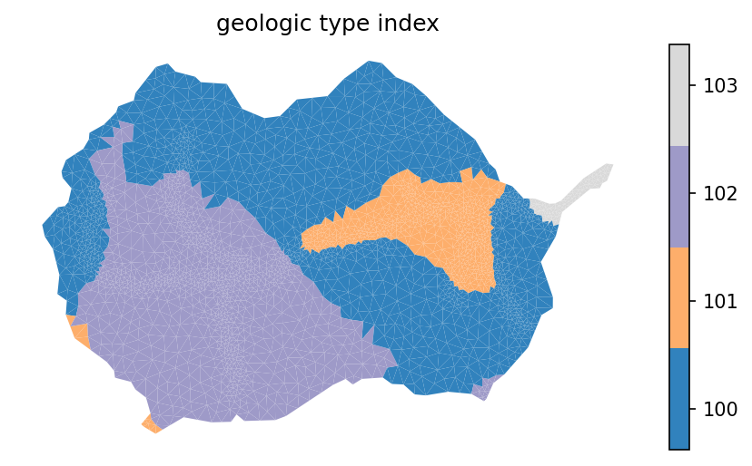
Depth-to-bedrock#
Depth to bedrock is taken from the SoilGrids product. Here we download a US-based, clipped version of this global product, as file sizes are quite large (all products potentially used total over 100GB).
DTB_profile, DTB_raster = watershed_workflow.get_raster_on_shape(sources['depth to bedrock'],
                                                                 watershed.exterior(), crs,
                                                                 nodata=-99999)
                                        #, variable='BDTICM') # note, this argument needed for
                                        # using the default SoilGrids dataset.

# resample the raster to the triangles
DTB_raster = DTB_raster/100 #convert from cm to m
DTB = watershed_workflow.values_from_raster(m2.centroids, crs, DTB_raster, DTB_profile, algorithm='piecewise bilinear')
DTB = np.where(DTB >= 0, DTB, np.nan)
2025-07-12 18:36:59,241 - root - INFO:
2025-07-12 18:36:59,244 - root - INFO: Loading Raster
2025-07-12 18:36:59,246 - root - INFO: ------------------------------
2025-07-12 18:36:59,250 - root - INFO: Collecting raster
2025-07-12 18:36:59,308 - root - INFO: bounds in my_crs: (-107.10634327399998, 38.82770288200003, -106.97736783099998, 38.89466788700003)
2025-07-12 18:36:59,314 - root - INFO: ... got raster of shape: (33, 63)
2025-07-12 18:36:59,324 - root - INFO: ... got raster bounds: (-107.10834499599999, 38.895007756000005, -106.97709501699998, 38.82625776700001)
# plot the resulting surface mesh
fig, ax = watershed_workflow.plot.get_ax(crs)

mp = watershed_workflow.plot.triangulation(mesh_points3, mesh_tris, crs, ax=ax,
                                 color=DTB, cmap='plasma_r', edgecolor='white', linewidth=0.1)
cbar = fig.colorbar(mp)
title = ax.set_title('DTB [m]')
ax.axis('off')
(316690.15495, 329034.55405000004, 4299344.3309, 4307420.0490999995)
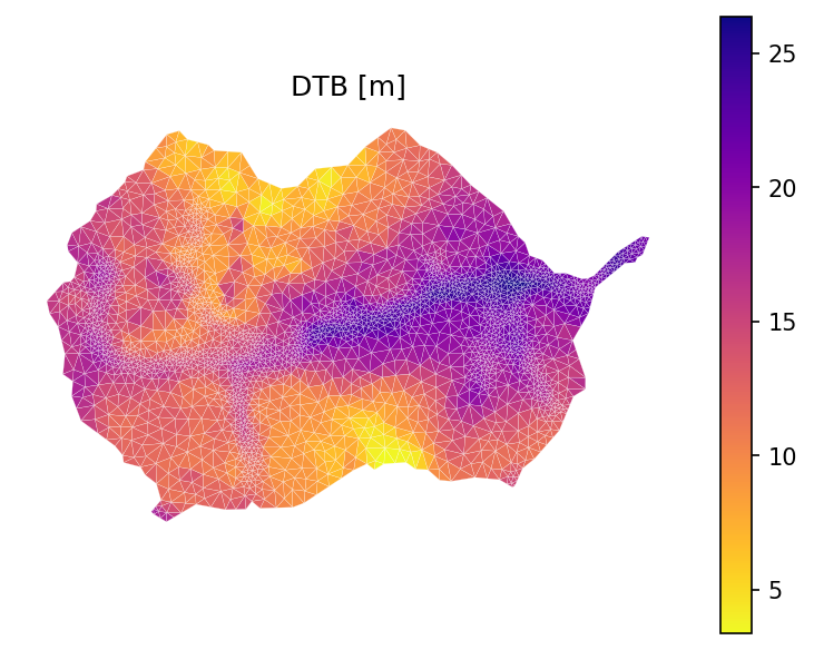
Mesh extrusion#
Given the surface mesh and material IDs on both the surface and subsurface, we can extrude the surface mesh in the vertical to make a 3D mesh.
First, all integer IDs in Exodus files must be unique. This includes Material IDs, side sets, etc. We create the Material ID map and data frame. This is used to standardize IDs from multiple data sources. Traditionally, ATS numbers Material IDs/Side Sets as:
0-9 : reserved for boundaries, surface/bottom, etc
10-99 : Land Cover side sets, typically NLCD IDs are used
100-999 : geologic layer material IDs
1000-9999 : soil layer material IDs
# map SSURGO mukey to ATS_ID
soil_survey_props_clean['ats_id'] = range(1000, 1000+len(soil_survey_props_clean))
soil_survey_props_clean.set_index('ats_id', inplace=True)

# map GLHYMPS id to ATS_ID
geo_survey_props_clean['ats_id'] = range(100, 100+len(geo_survey_props_clean))
geo_survey_props_clean.set_index('ats_id', inplace=True)
bedrock_props = watershed_workflow.soil_properties.get_bedrock_properties()
bedrock_props['source'] = 'SoilGrids'
bedrock_props['native_index'] = '(999,)'
# merge the properties databases
subsurface_props = pandas.concat([geo_survey_props_clean,
                                  soil_survey_props_clean,
                                  bedrock_props])
subsurface_props
| native_index | source | permeability [m^2] | porosity [-] | van Genuchten alpha [Pa^-1] | van Genuchten n [-] | residual saturation [-] | thickness [m] | |
|---|---|---|---|---|---|---|---|---|
| ats_id | ||||||||
| 100 | (715639, 715796, 726604, 726608) | GLHYMPS | 6.309573e-16 | 0.190000 | 0.000025 | 2.000000 | 0.010000 | NaN |
| 101 | (715779, 726642, 726664) | GLHYMPS | 3.162278e-13 | 0.090000 | 0.000817 | 2.000000 | 0.010000 | NaN |
| 102 | (715766, 726639, 726667) | GLHYMPS | 1.000000e-13 | 0.220000 | 0.000294 | 2.000000 | 0.010000 | NaN |
| 103 | (730801,) | GLHYMPS | 3.019952e-11 | 0.010000 | 0.023953 | 2.000000 | 0.010000 | NaN |
| 1000 | (509733,) | NRCS | 2.279759e-13 | 0.265563 | 0.000092 | 1.319916 | 0.240269 | 1.520000 |
| 1001 | (509477,) | NRCS | 2.734080e-12 | 0.159737 | 0.000139 | 1.457559 | 0.181598 | 1.520000 |
| 1002 | (498205, 498206) | NRCS | 1.184189e-12 | 0.185986 | 0.000071 | 1.420938 | 0.208316 | 1.520000 |
| 1003 | (509548,) | NRCS | 7.331979e-13 | 0.403218 | 0.000059 | 1.416784 | 0.213285 | 1.070000 |
| 1004 | (509529,) | NRCS | 3.039095e-12 | 0.428779 | 0.000103 | 1.383180 | 0.175133 | 1.520000 |
| 1005 | (509532,) | NRCS | 3.172415e-12 | 0.378365 | 0.000079 | 1.374540 | 0.230885 | 1.250000 |
| 1006 | (509482,) | NRCS | 4.654687e-12 | 0.369886 | 0.000092 | 1.397760 | 0.207877 | 1.205000 |
| 1007 | (498208,) | NRCS | 9.122162e-13 | 0.237423 | 0.000072 | 1.395746 | 0.219597 | 1.520000 |
| 1008 | (509559,) | NRCS | 2.375523e-13 | 0.271630 | 0.000079 | 1.340429 | 0.241801 | 1.520000 |
| 1009 | (498231,) | NRCS | 5.850942e-12 | 0.356163 | 0.000157 | 1.406091 | 0.196811 | 1.520000 |
| 1010 | (509513,) | NRCS | 1.526682e-12 | 0.182238 | 0.000087 | 1.422578 | 0.199783 | 1.520000 |
| 1011 | (509794,) | NRCS | 2.006536e-12 | 0.193350 | 0.000104 | 1.433685 | 0.189314 | 1.520000 |
| 1012 | (509479, 509481) | NRCS | 7.504374e-13 | 0.151250 | 0.000078 | 1.410010 | 0.210870 | 0.618125 |
| 1013 | (498185,) | NRCS | 1.590777e-13 | 0.218625 | 0.000081 | 1.332817 | 0.246665 | 1.396471 |
| 1014 | (509514,) | NRCS | 5.262229e-12 | 0.449752 | 0.000221 | 1.762072 | 0.157366 | 0.860000 |
| 1015 | (509561,) | NRCS | 1.554090e-12 | 0.415245 | 0.000140 | 1.367408 | 0.220962 | 1.520000 |
| 999 | (999,) | SoilGrids | 1.000000e-16 | 0.050000 | 0.000019 | 3.000000 | 0.010000 | NaN |
# save the properties to disk for use in generating input file
config['subsurface_properties_filename'] = os.path.join('..', '..', 'data', 'examples',watershed_name, 'processed', 'watershed_subsurface_properties.csv')
subsurface_props.to_csv(config['subsurface_properties_filename'])
Next we extrude the DEM to create a 3D mesh.
The most difficult aspect of extrusion is creating meshes that:
aren’t huge numbers of cells
aren’t huge cell thicknesses, especially near the surface
follow implied interfaces, e.g. bottom of soil and bottom of geologic layer
This is an iterative process that requires some care and some art.
# here we choose the bottom of the domain to be the maximum of the depth to bedrock.
# This is really up to the user, but we are hard-coding this for this watershed_workflow.
total_thickness = np.ceil(DTB.max())
logging.info(f'max DTB: {total_thickness} m')
2025-07-12 18:37:02,031 - root - INFO: max DTB: 27.0 m
# Generate a dz structure for the top 2m of soil -- it appears from above that the soil thickness is uniformly 2m
#
# here we try for 10 cells, starting at 5cm at the top and going to 50cm at the bottom of the 2m thick soil
dzs, res = watershed_workflow.mesh.optimize_dzs(0.05, 0.5, 2, 10)
print(dzs)
[0.05723957 0.07235405 0.10008891 0.1503918  0.24391084 0.37797867
 0.49803617 0.5       ]
# this looks like it would work out:
dzs_soil = [0.05, 0.05, 0.05, 0.12, 0.23, 0.5, 0.5, 0.5]
# a 2 m soil thickness and a maximum of 27 m depth to bedrock suggests a
# geologic layer of 13 * 2 m cells or something finer
dzs_geo = [2.0]*13
assert np.sum(dzs_soil) + np.sum(dzs_geo) > total_thickness, "The sum of soil and geology layers should be greater than the total thickness!"
# layer extrusion
# -- data structures needed for extrusion
layer_types = []
layer_data = []
layer_ncells = []
layer_mat_ids = []

# -- soil layer --
depth = 0
for dz in dzs_soil:
    depth += 0.5 * dz
    layer_types.append('constant')
    layer_data.append(dz)
    layer_ncells.append(1)

    br_or_geo = np.where(depth < DTB, geo_color_new, 999)
    soil_or_br_or_geo = np.where(np.bitwise_and(soil_color_new > 0, depth < soil_thickness),
                                 soil_color_new,
                                 br_or_geo)

    layer_mat_ids.append(soil_or_br_or_geo)
    depth += 0.5 * dz

# -- geologic layer --
for dz in dzs_geo:
    depth += 0.5 * dz
    layer_types.append('constant')
    layer_data.append(dz)
    layer_ncells.append(1)
    layer_mat_ids.append(np.where(depth < DTB, geo_color_new, 999))
    depth += 0.5 * dz

# print the summary
watershed_workflow.mesh.Mesh3D.summarize_extrusion(layer_types, layer_data,
                                            layer_ncells, layer_mat_ids)
2025-07-12 18:37:03,613 - root - INFO: Cell summary:
2025-07-12 18:37:03,615 - root - INFO: ------------------------------------------------------------
2025-07-12 18:37:03,618 - root - INFO: l_id	| c_id	|mat_id	| dz		| z_top
2025-07-12 18:37:03,621 - root - INFO: ------------------------------------------------------------
2025-07-12 18:37:03,625 - root - INFO:  00 	| 00 	| 1003 	|   0.050000 	|   0.000000
2025-07-12 18:37:03,629 - root - INFO:  01 	| 01 	| 1003 	|   0.050000 	|   0.050000
2025-07-12 18:37:03,631 - root - INFO:  02 	| 02 	| 1003 	|   0.050000 	|   0.100000
2025-07-12 18:37:03,633 - root - INFO:  03 	| 03 	| 1003 	|   0.120000 	|   0.150000
2025-07-12 18:37:03,635 - root - INFO:  04 	| 04 	| 1003 	|   0.230000 	|   0.270000
2025-07-12 18:37:03,637 - root - INFO:  05 	| 05 	| 1003 	|   0.500000 	|   0.500000
2025-07-12 18:37:03,639 - root - INFO:  06 	| 06 	| 1003 	|   0.500000 	|   1.000000
2025-07-12 18:37:03,641 - root - INFO:  07 	| 07 	|  102 	|   0.500000 	|   1.500000
2025-07-12 18:37:03,642 - root - INFO:  08 	| 08 	|  102 	|   2.000000 	|   2.000000
2025-07-12 18:37:03,645 - root - INFO:  09 	| 09 	|  102 	|   2.000000 	|   4.000000
2025-07-12 18:37:03,647 - root - INFO:  10 	| 10 	|  102 	|   2.000000 	|   6.000000
2025-07-12 18:37:03,653 - root - INFO:  11 	| 11 	|  102 	|   2.000000 	|   8.000000
2025-07-12 18:37:03,655 - root - INFO:  12 	| 12 	|  102 	|   2.000000 	|  10.000000
2025-07-12 18:37:03,657 - root - INFO:  13 	| 13 	|  102 	|   2.000000 	|  12.000000
2025-07-12 18:37:03,658 - root - INFO:  14 	| 14 	|  102 	|   2.000000 	|  14.000000
2025-07-12 18:37:03,661 - root - INFO:  15 	| 15 	|  999 	|   2.000000 	|  16.000000
2025-07-12 18:37:03,663 - root - INFO:  16 	| 16 	|  999 	|   2.000000 	|  18.000000
2025-07-12 18:37:03,665 - root - INFO:  17 	| 17 	|  999 	|   2.000000 	|  20.000000
2025-07-12 18:37:03,667 - root - INFO:  18 	| 18 	|  999 	|   2.000000 	|  22.000000
2025-07-12 18:37:03,673 - root - INFO:  19 	| 19 	|  999 	|   2.000000 	|  24.000000
2025-07-12 18:37:03,674 - root - INFO:  20 	| 20 	|  999 	|   2.000000 	|  26.000000
# extrude
m3 = watershed_workflow.mesh.Mesh3D.extruded_Mesh2D(m2, layer_types, layer_data,
                                             layer_ncells, layer_mat_ids)
# # add back on land cover side sets
# surf_ss = m3.side_sets[1]

# for index, name in zip(nlcd_indices, nlcd_labels):
#     where = np.where(lc == index)[0]
#     ss = watershed_workflow.mesh.SideSet(name, int(index),
#                             [surf_ss.cell_list[w] for w in where],
#                             [surf_ss.side_list[w] for w in where])
#     m3.side_sets.append(ss)
print(f'total number of cells: {m3.num_cells}')
print('---------------')
print('2D labeled sets')
print('---------------')
for ls in m2.labeled_sets:
    print(f'{ls.setid} : {ls.entity} : {len(ls.ent_ids)} : "{ls.name}"')

print('')
print('Extruded 3D labeled sets')
print('------------------------')
ls = {}
for i in m3.labeled_sets:
    ls[i.name] = {'setid':i.setid, 'entity':i.entity}
    print(f'{i.setid} : {i.entity} : {len(i.ent_ids)} : "{i.name}"')

print('')
print('Extruded 3D side sets')
print('---------------------')
ss = {}
for i in m3.side_sets:
    ss[i.name] = {'setid':i.setid}
    print(f'{i.setid} : FACE : {len(i.cell_list)} : "{i.name}"')
total number of cells: 100653
---------------
2D labeled sets
---------------
10000 : CELL : 4793 : "140200010204"
10001 : CELL : 4793 : "140200010204 surface"
10002 : FACE : 177 : "140200010204 boundary"
10003 : FACE : 12 : "140200010204 outlet"
10004 : FACE : 12 : "surface domain outlet"
8 : CELL : 3057 : "Woody Savannas"
9 : CELL : 156 : "Savannas"
10 : CELL : 1580 : "Grasslands"

Extruded 3D labeled sets
------------------------
10000 : CELL : 100653 : "140200010204"

Extruded 3D side sets
---------------------
1 : FACE : 4793 : "bottom"
2 : FACE : 4793 : "surface"
3 : FACE : 3717 : "external_sides"
10001 : FACE : 4793 : "140200010204 surface"
10002 : FACE : 3717 : "140200010204 boundary"
10003 : FACE : 252 : "140200010204 outlet"
10004 : FACE : 252 : "surface domain outlet"
8 : FACE : 3057 : "Woody Savannas"
9 : FACE : 156 : "Savannas"
10 : FACE : 1580 : "Grasslands"
config['labeled_sets'] = ls
config['side_sets'] = ss
Save mesh file#
This will write the 3D mesh to ExodusII using arbitrary polyhedra specification.
config['mesh_filename'] = os.path.join('..', '..', 'data', 'examples',watershed_name, 'processed','watershed_mesh.exo')

try:
    os.remove(config['mesh_filename'])
except FileNotFoundError:
    pass
m3.write_exodus(config['mesh_filename'])
You are using exodus.py v 1.20.10 (seacas-py3), a python wrapper of some of the exodus library.

Copyright (c) 2013, 2014, 2015, 2016, 2017, 2018, 2019, 2020, 2021 National Technology &
Engineering Solutions of Sandia, LLC (NTESS).  Under the terms of
Contract DE-NA0003525 with NTESS, the U.S. Government retains certain
rights in this software.

Opening exodus file: ../../data/examples/CoalCreek/processed/watershed_mesh.exo
2025-07-12 18:37:38,495 - root - INFO: adding side set: 1
2025-07-12 18:37:39,595 - root - INFO: adding side set: 2
2025-07-12 18:37:40,736 - root - INFO: adding side set: 3
2025-07-12 18:37:41,853 - root - INFO: adding side set: 10001
2025-07-12 18:37:42,974 - root - INFO: adding side set: 10002
2025-07-12 18:37:44,129 - root - INFO: adding side set: 10003
2025-07-12 18:37:45,277 - root - INFO: adding side set: 10004
2025-07-12 18:37:46,392 - root - INFO: adding side set: 8
2025-07-12 18:37:47,521 - root - INFO: adding side set: 9
2025-07-12 18:37:48,621 - root - INFO: adding side set: 10
2025-07-12 18:37:50,056 - root - INFO: adding elem set: 10000
Closing exodus file: ../../data/examples/CoalCreek/processed/watershed_mesh.exo
config['start_date'] = start_date
config['end_date'] = end_date
config['origin_date'] = origin_date
config['nyears_cyclic_steadystate'] = nyears_cyclic_steadystate
config
{'catchment_labels': ['140200010204'],
 'nlcd_indices': [8, 9, 10],
 'nlcd_labels': ['Woody Savannas', 'Savannas', 'Grasslands'],
 'LAI_filename': '../../data/examples/CoalCreek/processed/watershed_lai_raw.h5',
 'LAI_typical_filename': '../../data/examples/CoalCreek/processed/watershed_lai_typical.h5',
 'subsurface_properties_filename': '../../data/examples/CoalCreek/processed/watershed_subsurface_properties.csv',
 'labeled_sets': {'140200010204': {'setid': 10000, 'entity': 'CELL'}},
 'side_sets': {'bottom': {'setid': 1},
  'surface': {'setid': 2},
  'external_sides': {'setid': 3},
  '140200010204 surface': {'setid': 10001},
  '140200010204 boundary': {'setid': 10002},
  '140200010204 outlet': {'setid': 10003},
  'surface domain outlet': {'setid': 10004},
  'Woody Savannas': {'setid': 8},
  'Savannas': {'setid': 9},
  'Grasslands': {'setid': 10}},
 'mesh_filename': '../../data/examples/CoalCreek/processed/watershed_mesh.exo',
 'start_date': '2015-10-1',
 'end_date': '2017-10-1',
 'origin_date': '1980-1-1',
 'nyears_cyclic_steadystate': 4}
# Save dictionary to a file
# config['config_file'] = os.path.join('..', '..', 'data', 'examples',watershed_name, 'processed','config.yaml')

with open(config_fname, 'w') as file:
    yaml.dump(config, file)